Analysis of young samples
Belinda Phipson
20 June 2019
Last updated: 2019-07-05
Checks: 6 0
Knit directory: Porello-heart-snRNAseq/
This reproducible R Markdown analysis was created with workflowr (version 1.3.0). The Checks tab describes the reproducibility checks that were applied when the results were created. The Past versions tab lists the development history.
Great! Since the R Markdown file has been committed to the Git repository, you know the exact version of the code that produced these results.
Great job! The global environment was empty. Objects defined in the global environment can affect the analysis in your R Markdown file in unknown ways. For reproduciblity it’s best to always run the code in an empty environment.
The command set.seed(20190603) was run prior to running the code in the R Markdown file. Setting a seed ensures that any results that rely on randomness, e.g. subsampling or permutations, are reproducible.
Great job! Recording the operating system, R version, and package versions is critical for reproducibility.
Nice! There were no cached chunks for this analysis, so you can be confident that you successfully produced the results during this run.
Great! You are using Git for version control. Tracking code development and connecting the code version to the results is critical for reproducibility. The version displayed above was the version of the Git repository at the time these results were generated.
Note that you need to be careful to ensure that all relevant files for the analysis have been committed to Git prior to generating the results (you can use wflow_publish or wflow_git_commit). workflowr only checks the R Markdown file, but you know if there are other scripts or data files that it depends on. Below is the status of the Git repository when the results were generated:
Ignored files:
    Ignored:    .Rhistory
    Ignored:    .Rproj.user/

Untracked files:
    Untracked:  analysis/05-ClusterDCM.Rmd
    Untracked:  code/ReadDataObjects.R
    Untracked:  data/gstlist-fetal.Rdata
    Untracked:  data/gstlist-young.Rdata
    Untracked:  data/heart-markers-long.txt
    Untracked:  data/pseudobulk.Rds
    Untracked:  output/AllAdult-clustermarkers.csv
    Untracked:  output/AllFetal-clustermarkers.csv
    Untracked:  output/AllYoung-clustermarkers.csv
    Untracked:  output/Alldcm-clustermarkers.csv
    Untracked:  output/Figures/
    Untracked:  output/MarkerAnalysis/
    Untracked:  output/RDataObjects/
    Untracked:  output/fetal1-clustermarkers.csv
    Untracked:  output/fetal2-clustermarkers.csv
    Untracked:  output/fetal3-clustermarkers.csv
    Untracked:  output/heatmap-top10-adultmarkergenes.pdf
    Untracked:  output/young1-clustermarkers.csv

Unstaged changes:
    Modified:   analysis/01-QualityControl.Rmd
    Modified:   analysis/01a-DEpseudobulk.Rmd
    Modified:   analysis/02-ClusterFetal.Rmd
    Modified:   analysis/02c-ClusterFetal3.Rmd
Note that any generated files, e.g. HTML, png, CSS, etc., are not included in this status report because it is ok for generated content to have uncommitted changes.
These are the previous versions of the R Markdown and HTML files. If you’ve configured a remote Git repository (see ?wflow_git_remote), click on the hyperlinks in the table below to view them.
| File | Version | Author | Date | Message |
|---|---|---|---|---|
| Rmd | da40aba | Belinda Phipson | 2019-07-05 | update young and adult analysis |
| html | b0f9c92 | Belinda Phipson | 2019-07-04 | Build site. |
| Rmd | e590fe0 | Belinda Phipson | 2019-07-04 | update fetal and young integrated analysis |
| html | 45c47f7 | Belinda Phipson | 2019-06-20 | Build site. |
| Rmd | c5fd8ad | Belinda Phipson | 2019-06-20 | add new integrated clustering analysis of young samples |
Introduction
I will cluster all the young samples from batch 1 and batch 2 using the integration technique from the Seurat package.
I am taking the same approach as I did for the fetal samples:
- Remove mitochondrial, ribosomal and genes with no annotation
- Gene filtering of lowly expressed genes assuming min cluster size of 20
- Remove genes on X and Y chromosome so they are not selected to perform clustering
- Use SCTransform to normalise the data without including additional covariates
- Perform data integration across biological replicates
- Use 30 CCA dimensions
- Use 3000 anchor features
- Scale data
- Run principle components analysis
- Perform clustering
- Use 20 CCA dimensions
- Resolution = 0.3 for marker analysis
- Visualisation with TSNE and clustree
- Marker analysis
Load libraries and functions
library(edgeR)Loading required package: limmalibrary(RColorBrewer)
library(org.Hs.eg.db)Loading required package: AnnotationDbiLoading required package: stats4Loading required package: BiocGenericsLoading required package: parallel
Attaching package: 'BiocGenerics'The following objects are masked from 'package:parallel':
clusterApply, clusterApplyLB, clusterCall, clusterEvalQ,
clusterExport, clusterMap, parApply, parCapply, parLapply,
parLapplyLB, parRapply, parSapply, parSapplyLBThe following object is masked from 'package:limma':
plotMAThe following objects are masked from 'package:stats':
IQR, mad, sd, var, xtabsThe following objects are masked from 'package:base':
anyDuplicated, append, as.data.frame, basename, cbind,
colnames, dirname, do.call, duplicated, eval, evalq, Filter,
Find, get, grep, grepl, intersect, is.unsorted, lapply, Map,
mapply, match, mget, order, paste, pmax, pmax.int, pmin,
pmin.int, Position, rank, rbind, Reduce, rownames, sapply,
setdiff, sort, table, tapply, union, unique, unsplit, which,
which.max, which.minLoading required package: BiobaseWelcome to Bioconductor
Vignettes contain introductory material; view with
'browseVignettes()'. To cite Bioconductor, see
'citation("Biobase")', and for packages 'citation("pkgname")'.Loading required package: IRangesLoading required package: S4Vectors
Attaching package: 'S4Vectors'The following object is masked from 'package:base':
expand.gridlibrary(limma)
library(Seurat)Registered S3 method overwritten by 'R.oo':
method from
throw.default R.methodsS3Registered S3 methods overwritten by 'ggplot2':
method from
[.quosures rlang
c.quosures rlang
print.quosures rlanglibrary(monocle)Loading required package: Matrix
Attaching package: 'Matrix'The following object is masked from 'package:S4Vectors':
expandLoading required package: ggplot2Loading required package: VGAMLoading required package: splinesLoading required package: DDRTreeLoading required package: irlbalibrary(cowplot)
Attaching package: 'cowplot'The following object is masked from 'package:ggplot2':
ggsavelibrary(DelayedArray)Loading required package: matrixStats
Attaching package: 'matrixStats'The following objects are masked from 'package:Biobase':
anyMissing, rowMediansLoading required package: BiocParallel
Attaching package: 'DelayedArray'The following objects are masked from 'package:matrixStats':
colMaxs, colMins, colRanges, rowMaxs, rowMins, rowRangesThe following objects are masked from 'package:base':
aperm, apply, rowsumlibrary(scran)Loading required package: SingleCellExperimentLoading required package: SummarizedExperimentLoading required package: GenomicRangesLoading required package: GenomeInfoDb
Attaching package: 'SingleCellExperiment'The following object is masked from 'package:edgeR':
cpmlibrary(NMF)Loading required package: pkgmakerLoading required package: registry
Attaching package: 'pkgmaker'The following object is masked from 'package:S4Vectors':
new2The following object is masked from 'package:base':
isFALSELoading required package: rngtoolsLoading required package: clusterNMF - BioConductor layer [OK] | Shared memory capabilities [NO: synchronicity] | Cores 31/32 To enable shared memory capabilities, try: install.extras('
NMF
')
Attaching package: 'NMF'The following object is masked from 'package:DelayedArray':
seedThe following object is masked from 'package:BiocParallel':
registerThe following object is masked from 'package:S4Vectors':
nrunlibrary(workflowr)This is workflowr version 1.3.0
Run ?workflowr for help getting startedlibrary(ggplot2)
library(clustree)Loading required package: ggraphlibrary(dplyr)
Attaching package: 'dplyr'The following objects are masked from 'package:GenomicRanges':
intersect, setdiff, unionThe following object is masked from 'package:GenomeInfoDb':
intersectThe following object is masked from 'package:matrixStats':
countThe following object is masked from 'package:AnnotationDbi':
selectThe following objects are masked from 'package:IRanges':
collapse, desc, intersect, setdiff, slice, unionThe following objects are masked from 'package:S4Vectors':
first, intersect, rename, setdiff, setequal, unionThe following object is masked from 'package:Biobase':
combineThe following objects are masked from 'package:BiocGenerics':
combine, intersect, setdiff, unionThe following objects are masked from 'package:stats':
filter, lagThe following objects are masked from 'package:base':
intersect, setdiff, setequal, unionsource("/misc/card2-single_cell_nuclei_rnaseq/Porello-heart-snRNAseq/code/normCounts.R")
source("/misc/card2-single_cell_nuclei_rnaseq/Porello-heart-snRNAseq/code/findModes.R")
source("/misc/card2-single_cell_nuclei_rnaseq/Porello-heart-snRNAseq/code/ggplotColors.R")Read in the young data
targets <- read.delim("/misc/card2-single_cell_nuclei_rnaseq/Porello-heart-snRNAseq/data/targets.txt",header=TRUE, stringsAsFactors = FALSE)
targets$FileName2 <- paste(targets$FileName,"/",sep="")
targets$Group_ID2 <- gsub("LV_","",targets$Group_ID)
group <- c("Fetal_1","Fetal_2","Fetal_3",
           "Young_1","Young_2","Young_3",
           "Adult_1","Adult_2","Adult_3",
           "Diseased_1","Diseased_2",
           "Diseased_3","Diseased_4")
m <- match(group, targets$Group_ID2)
targets <- targets[m,]
y1 <- Read10X(data.dir = targets$FileName2[targets$Group_ID2=="Young_1"])
colnames(y1) <- paste(colnames(y1),"y1",sep="_")
y2 <- Read10X(data.dir = targets$FileName2[targets$Group_ID2=="Young_2"])
colnames(y2) <- paste(colnames(y2),"y2",sep="_")
y3 <- Read10X(data.dir = targets$FileName2[targets$Group_ID2=="Young_3"])
colnames(y3) <- paste(colnames(y3),"y3",sep="_")
# Combine 3 samples into one big data matrix
ally <- cbind(y1,y2,y3)Gene filtering
Get gene annotation
I’m using gene annotation information from the org.Hs.eg.db package.
columns(org.Hs.eg.db) [1] "ACCNUM" "ALIAS" "ENSEMBL" "ENSEMBLPROT"
[5] "ENSEMBLTRANS" "ENTREZID" "ENZYME" "EVIDENCE"
[9] "EVIDENCEALL" "GENENAME" "GO" "GOALL"
[13] "IPI" "MAP" "OMIM" "ONTOLOGY"
[17] "ONTOLOGYALL" "PATH" "PFAM" "PMID"
[21] "PROSITE" "REFSEQ" "SYMBOL" "UCSCKG"
[25] "UNIGENE" "UNIPROT" ann <- AnnotationDbi:::select(org.Hs.eg.db,keys=rownames(ally),columns=c("SYMBOL","ENTREZID","ENSEMBL","GENENAME","CHR"),keytype = "SYMBOL")'select()' returned 1:many mapping between keys and columnsm <- match(rownames(ally),ann$SYMBOL)
ann <- ann[m,]
table(ann$SYMBOL==rownames(ally))
 TRUE
33939
mito <- grep("mitochondrial",ann$GENENAME)
length(mito)[1] 226ribo <- grep("ribosomal",ann$GENENAME)
length(ribo)[1] 198missingEZID <- which(is.na(ann$ENTREZID))
length(missingEZID)[1] 10530Remove mitochondrial and ribosomal genes and genes with no ENTREZID
These genes are not informative for downstream analysis.
chuck <- unique(c(mito,ribo,missingEZID))
length(chuck)
[1] 10875ally.keep <- ally[-chuck,]
ann.keep <- ann[-chuck,]
table(ann.keep$SYMBOL==rownames(ally.keep))
 TRUE
23064
Remove very lowly expressed genes
Removing very lowly expressed genes helps to reduce the noise in the data. Here I am choosing to keep genes with at least 1 count in at least 20 cells. This means that a cluster made up of at least 20 cells can potentially be detected (minimum cluster size = 20 cells).
numzero.genes <- rowSums(ally.keep==0)

#avg.exp <- rowMeans(cpm.DGEList(y.kid,log=TRUE))

#plot(avg.exp,numzero.genes,xlab="Average log-normalised-counts",ylab="Number zeroes per gene")

table(numzero.genes > (ncol(ally.keep)-20))
FALSE  TRUE
17823  5241
keep.genes <- numzero.genes < (ncol(ally.keep)-20)
table(keep.genes)keep.genes
FALSE TRUE
5313 17751 ally.keep <- ally.keep[keep.genes,]
dim(ally.keep)[1] 17751 16964ann.keep <- ann.keep[keep.genes,]The total size of the young dataset is 16964 cells and 17751 genes.
Remove sex chromosome genes
I will remove the sex chromosome genes before clustering so that the sex doesn’t play a role in determining the clusters.
sexchr <- ann.keep$CHR %in% c("X","Y")

ally.nosex <- ally.keep[!sexchr,]
dim(ally.nosex)
[1] 17095 16964ann.nosex <- ann.keep[!sexchr,]Save data objects
#save(ann,ann.keep,ann.nosex,ally,ally.keep,ally.nosex,file="./output/RDataObjects/youngObjs.Rdata")
#load(file="./output/RDataObjects/youngObjs.Rdata")
Create Seurat objects
Here I am following the Seurat vignette on performing clustering using their integration method to deal with batch effects.
biorep <- factor(rep(c("y1","y2","y3"),c(ncol(y1),ncol(y2),ncol(y3))))
names(biorep) <- colnames(ally.keep)
sex <- factor(rep(c("m","f","m"),c(ncol(y1),ncol(y2),ncol(y3))))
names(sex) <- colnames(ally.keep)
age <- rep(c(4,10,14),c(ncol(y1),ncol(y2),ncol(y3)))
names(age) <- colnames(ally.keep)
batch <- rep(c("B1","B2","B2"),c(ncol(y1),ncol(y2),ncol(y3)))
names(batch) <- colnames(ally.keep)
age <-rep(c(4,10,14),c(ncol(y1),ncol(y2),ncol(y3)))
names(age) <- colnames(ally.keep)

young <- CreateSeuratObject(counts = ally.nosex, project = "young")
young <- AddMetaData(object=young, metadata = biorep, col.name="biorep")
young <- AddMetaData(object=young, metadata = sex, col.name="sex")
young <- AddMetaData(object=young, metadata = age, col.name="age")
young <- AddMetaData(object=young, metadata = batch, col.name="batch")
young.list <- SplitObject(young, split.by = "biorep")Try new normalisation method: SCTransform
This new method replaces the NormalizeData, FindVariableFeatures and ScaleData functions. It performs regularised negative binomial regression with the total sequencing depth per cell as the covariate (i.e. library size), as well as any other user supplied covariates. The Pearson residuals are then used in downstream analysis.
# This is a bit slow
for (i in 1:length(young.list)) {
    young.list[[i]] <- SCTransform(young.list[[i]], verbose = FALSE)
#    young.list[[i]] <- GetResidual(young.list[[i]])
}
Perform the usual normalisation
#for (i in 1:length(young.list)) {
#    young.list[[i]] <- NormalizeData(young.list[[i]], verbose = FALSE)
#    young.list[[i]] <- FindVariableFeatures(young.list[[i]], selection.method #= "vst",
#                                            nfeatures = 2000, verbose = FALSE)
#}
Perform integration
There are two steps:
- Find integration anchors
- Perform integration which should batch-correct the data
young.anchors <- FindIntegrationAnchors(object.list = young.list, dims = 1:30, anchor.features = 3000)Computing 3000 integration featuresScaling features for provided objectsFinding all pairwise anchorsRunning CCAMerging objectsFinding neighborhoodsFinding anchors Found 9615 anchorsFiltering anchors Retained 5296 anchorsExtracting within-dataset neighborsRunning CCAMerging objectsFinding neighborhoodsFinding anchors Found 8672 anchorsFiltering anchors Retained 4584 anchorsExtracting within-dataset neighborsRunning CCAMerging objectsFinding neighborhoodsFinding anchors Found 8830 anchorsFiltering anchors Retained 4872 anchorsExtracting within-dataset neighborsyoung.integrated <- IntegrateData(anchorset = young.anchors, dims = 1:30)Merging dataset 1 into 2Extracting anchors for merged samplesFinding integration vectorsFinding integration vector weightsIntegrating dataMerging dataset 3 into 2 1Extracting anchors for merged samplesFinding integration vectorsFinding integration vector weightsIntegrating dataPerform clustering
DefaultAssay(object = young.integrated) <- "integrated"Perform scaling and PCA
young.integrated <- ScaleData(young.integrated, verbose = FALSE)
young.integrated <- RunPCA(young.integrated, npcs = 50, verbose = FALSE)
ElbowPlot(young.integrated,ndims=50)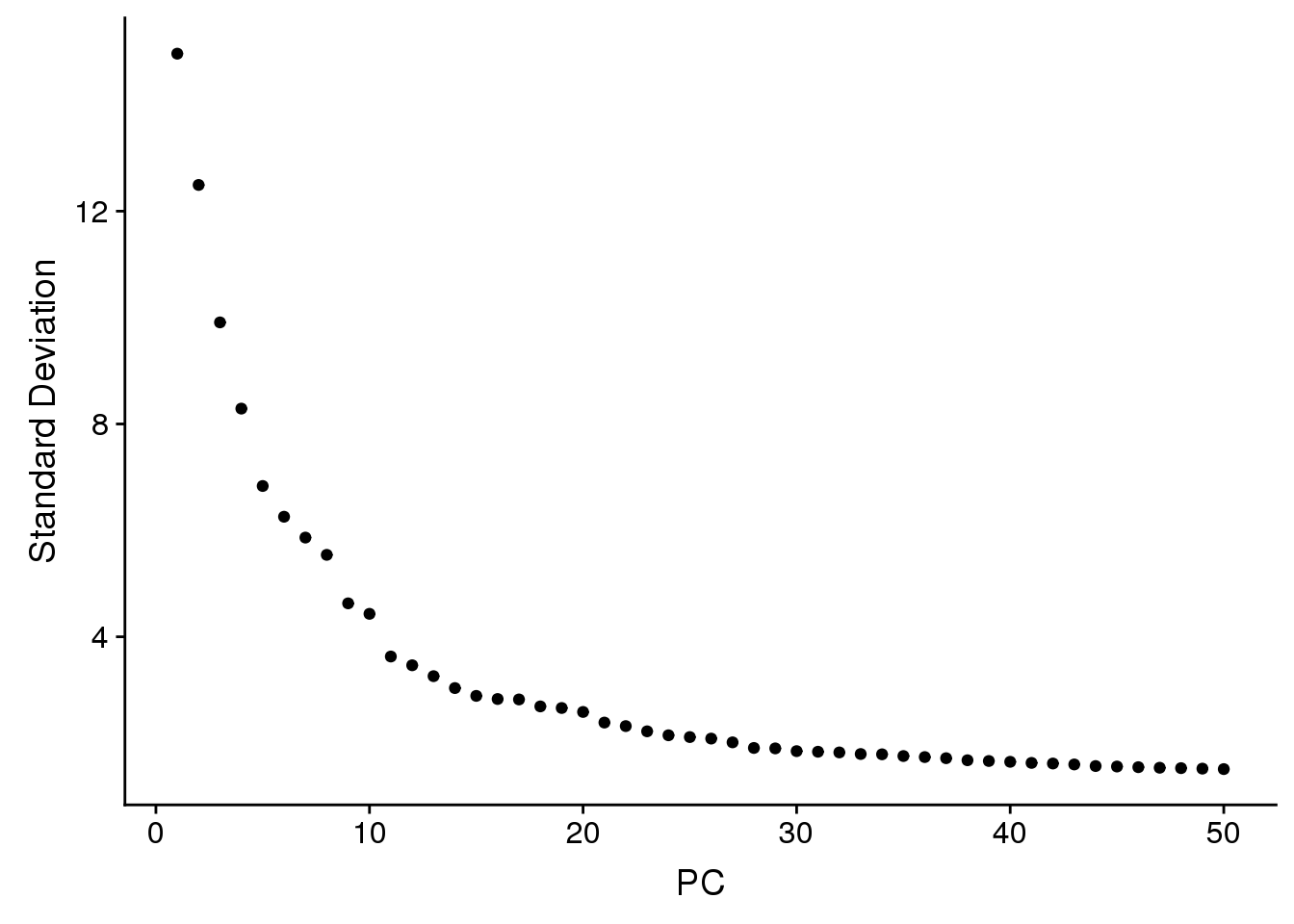
| Version | Author | Date |
|---|---|---|
| 45c47f7 | Belinda Phipson | 2019-06-20 |
VizDimLoadings(young.integrated, dims = 1:4, reduction = "pca")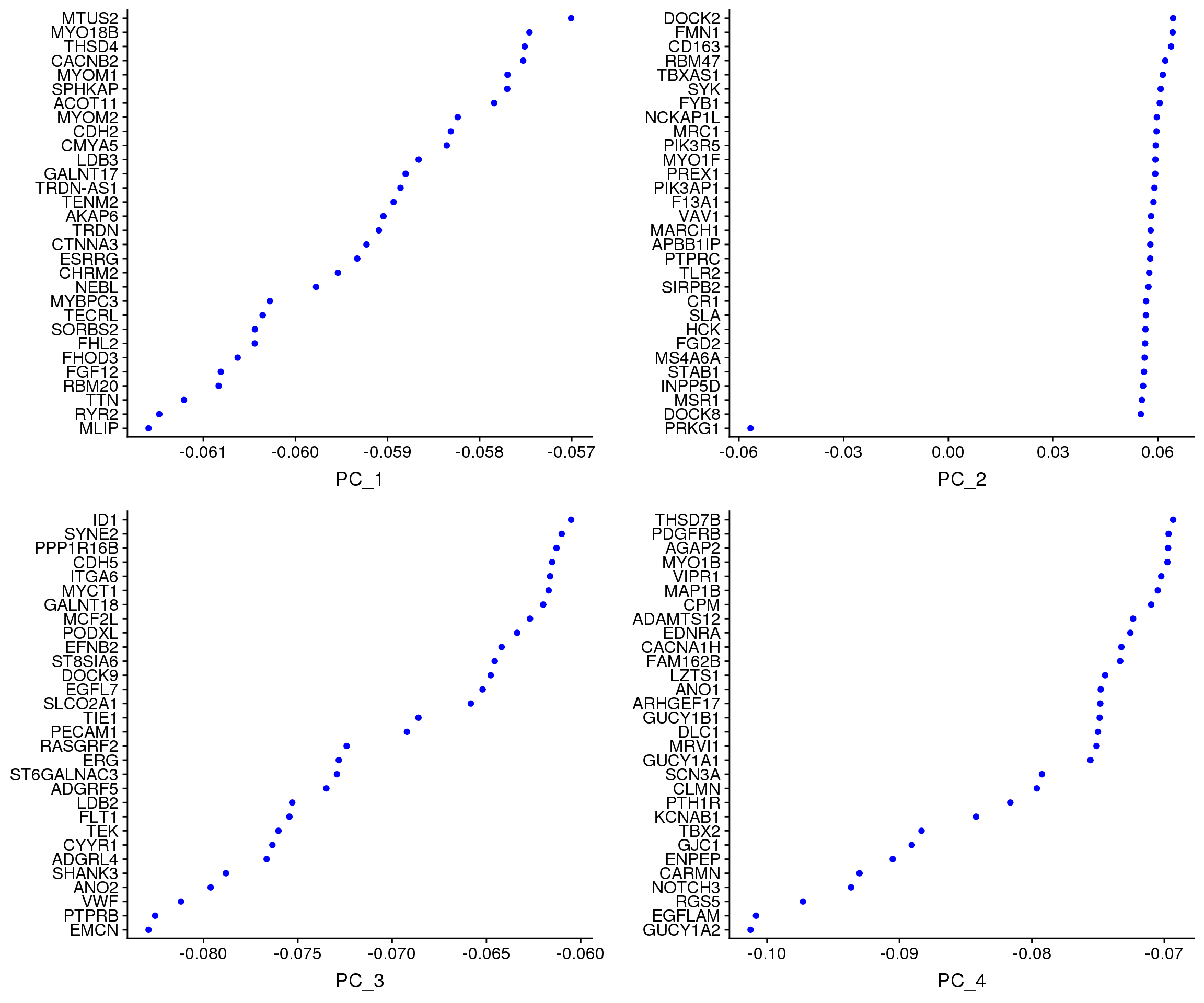
| Version | Author | Date |
|---|---|---|
| 45c47f7 | Belinda Phipson | 2019-06-20 |
DimPlot(young.integrated, reduction = "pca",group.by="biorep")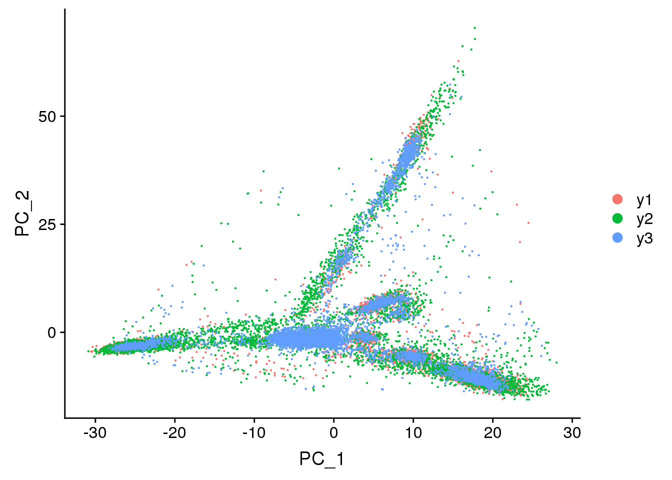
DimPlot(young.integrated, reduction = "pca",group.by="sex")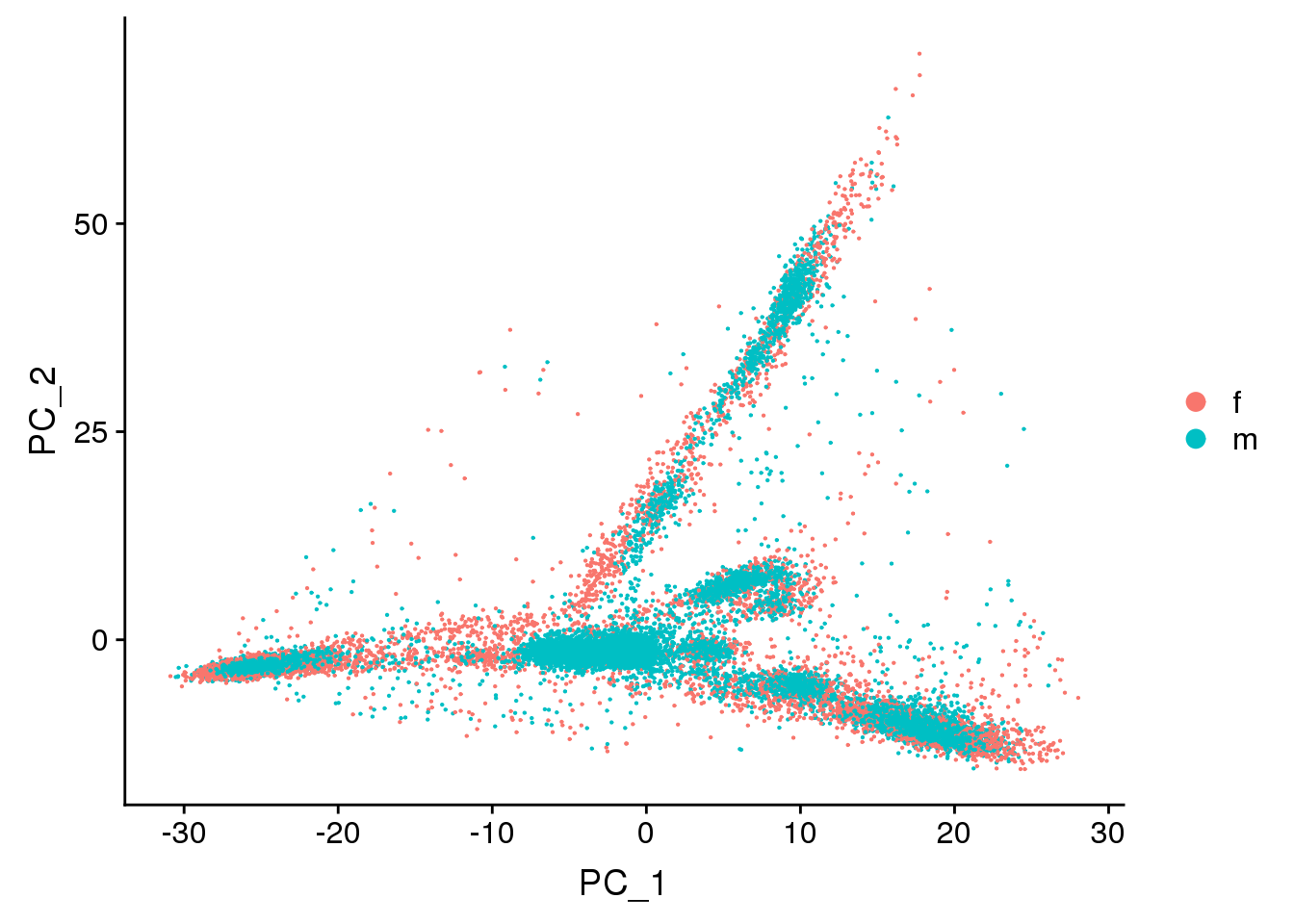
| Version | Author | Date |
|---|---|---|
| 45c47f7 | Belinda Phipson | 2019-06-20 |
DimPlot(young.integrated, reduction = "pca",group.by="batch")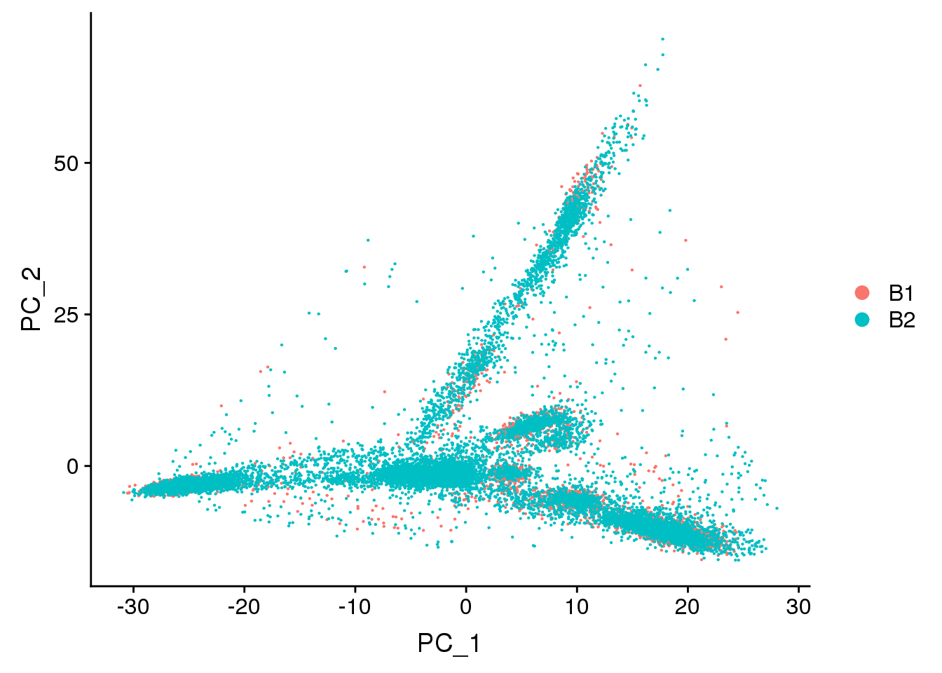
| Version | Author | Date |
|---|---|---|
| 45c47f7 | Belinda Phipson | 2019-06-20 |
DimHeatmap(young.integrated, dims = 1:15, cells = 500, balanced = TRUE)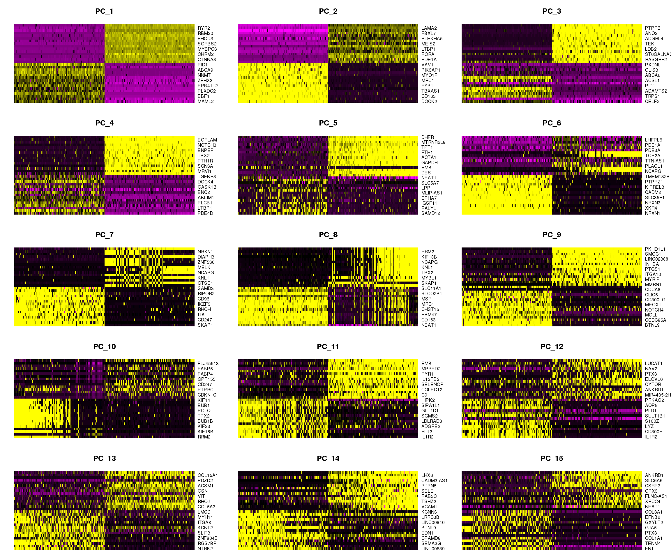
DimHeatmap(young.integrated, dims = 16:30, cells = 500, balanced = TRUE)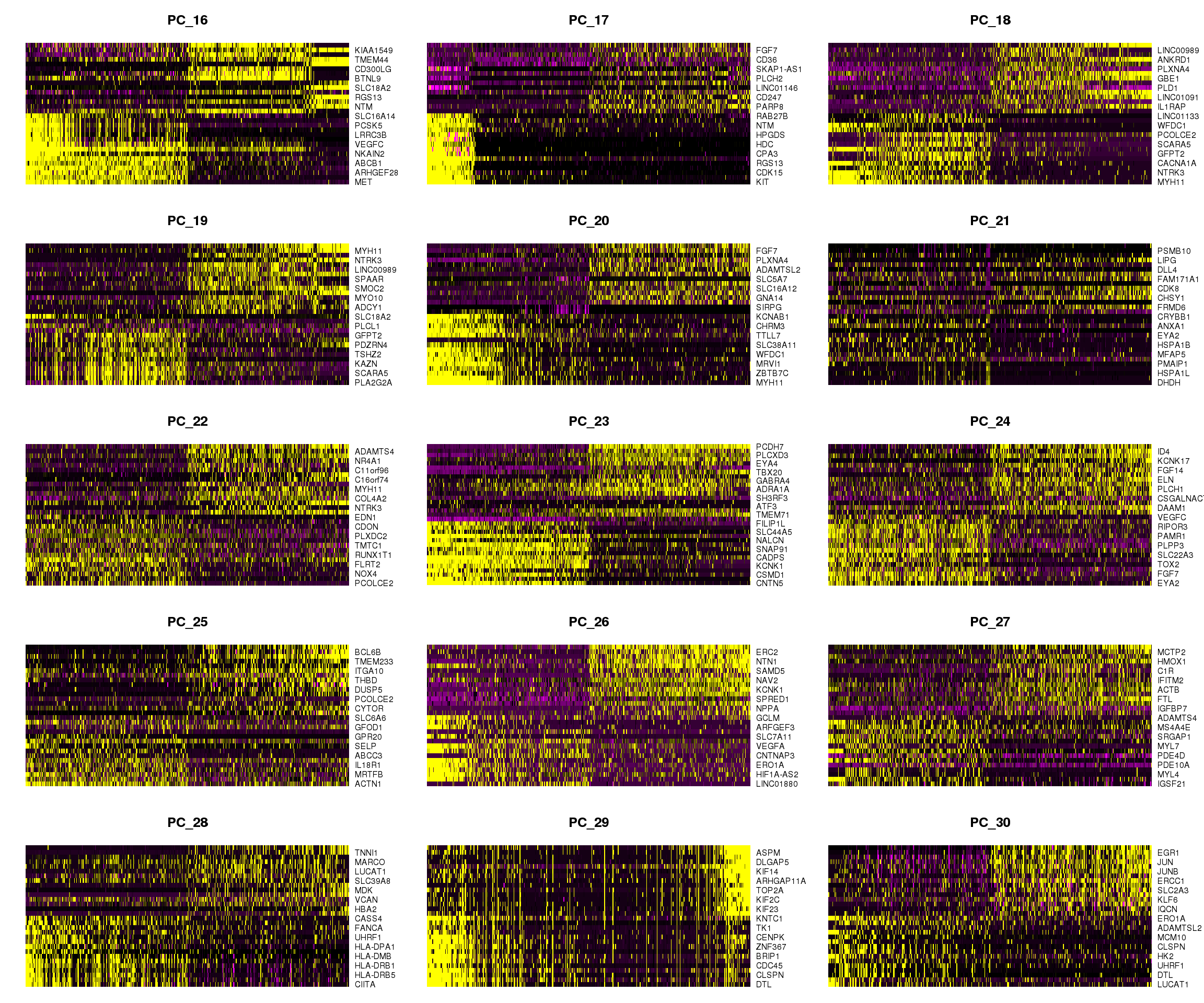
Perform nearest neighbours clustering
young.integrated <- FindNeighbors(young.integrated, dims = 1:20)Computing nearest neighbor graphComputing SNNyoung.integrated <- FindClusters(young.integrated, resolution = 0.3)Modularity Optimizer version 1.3.0 by Ludo Waltman and Nees Jan van Eck
Number of nodes: 16964
Number of edges: 692708
Running Louvain algorithm...
Maximum modularity in 10 random starts: 0.9543
Number of communities: 17
Elapsed time: 2 secondstable(Idents(young.integrated))
0 1 2 3 4 5 6 7 8 9 10 11 12 13 14
3713 2561 2445 1337 1325 1167 1153 794 513 411 402 360 356 136 126
15 16
100 65 barplot(table(Idents(young.integrated)),ylab="Number of cells",xlab="Clusters")
title("Number of cells in each cluster")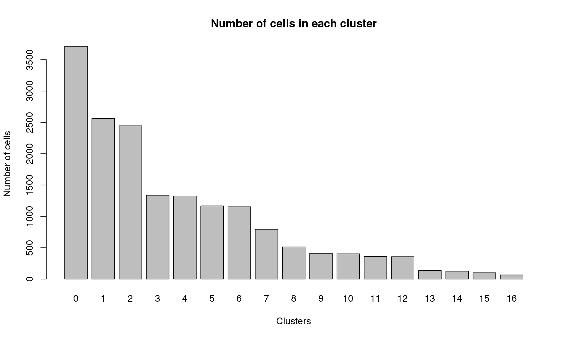
Visualisation with TSNE
set.seed(10)
young.integrated <- RunTSNE(young.integrated, reduction = "pca", dims = 1:20)pdf(file="./output/Figures/tsne-youngALL.pdf",width=10,height=8,onefile = FALSE)
DimPlot(young.integrated, reduction = "tsne",label=TRUE,label.size = 6,pt.size = 0.5)+NoLegend()
dev.off()png
2 DimPlot(young.integrated, reduction = "tsne",label=TRUE,label.size = 6)+NoLegend()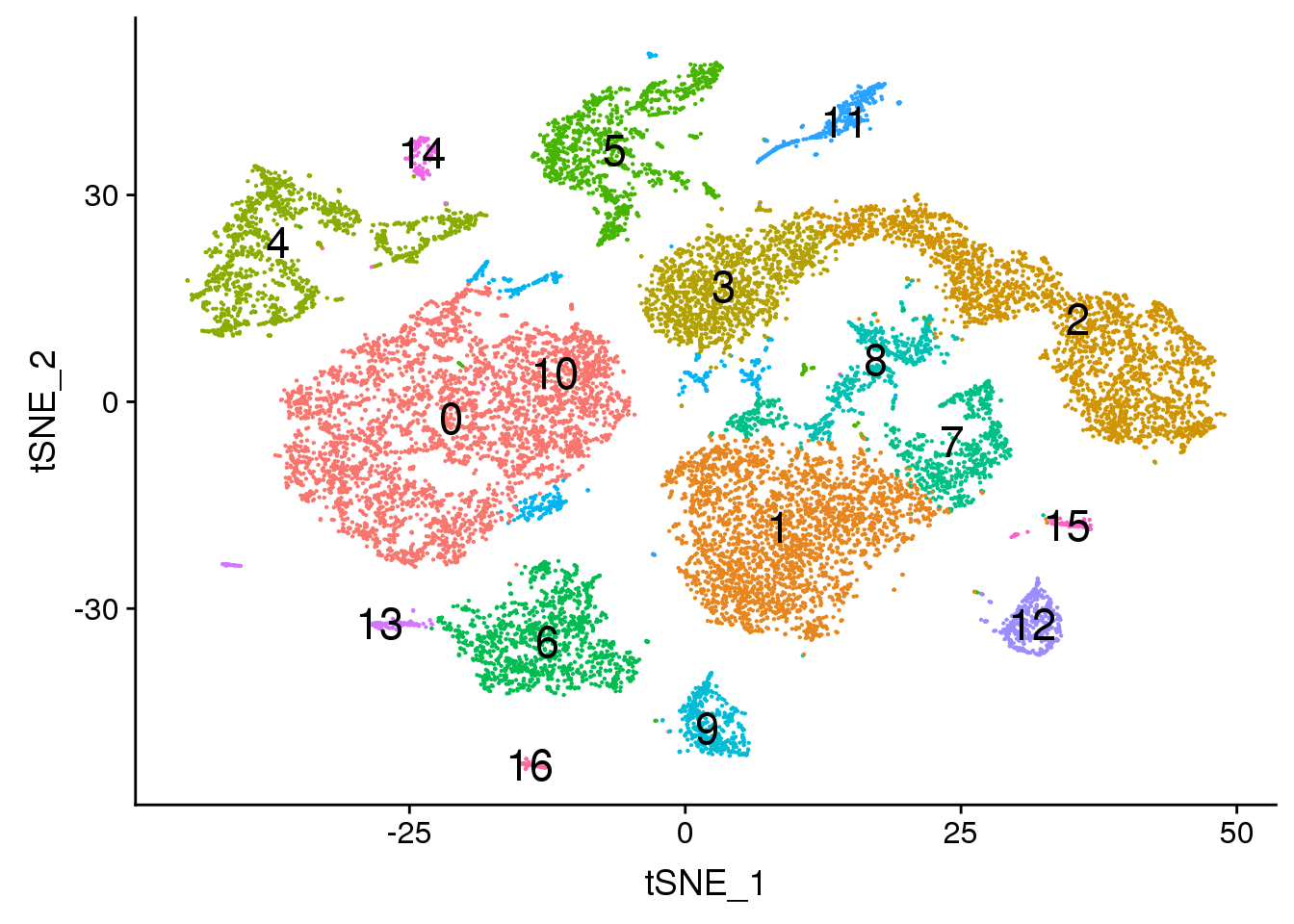
DimPlot(young.integrated, reduction = "tsne", split.by = "biorep",label=TRUE,label.size = 5)+NoLegend()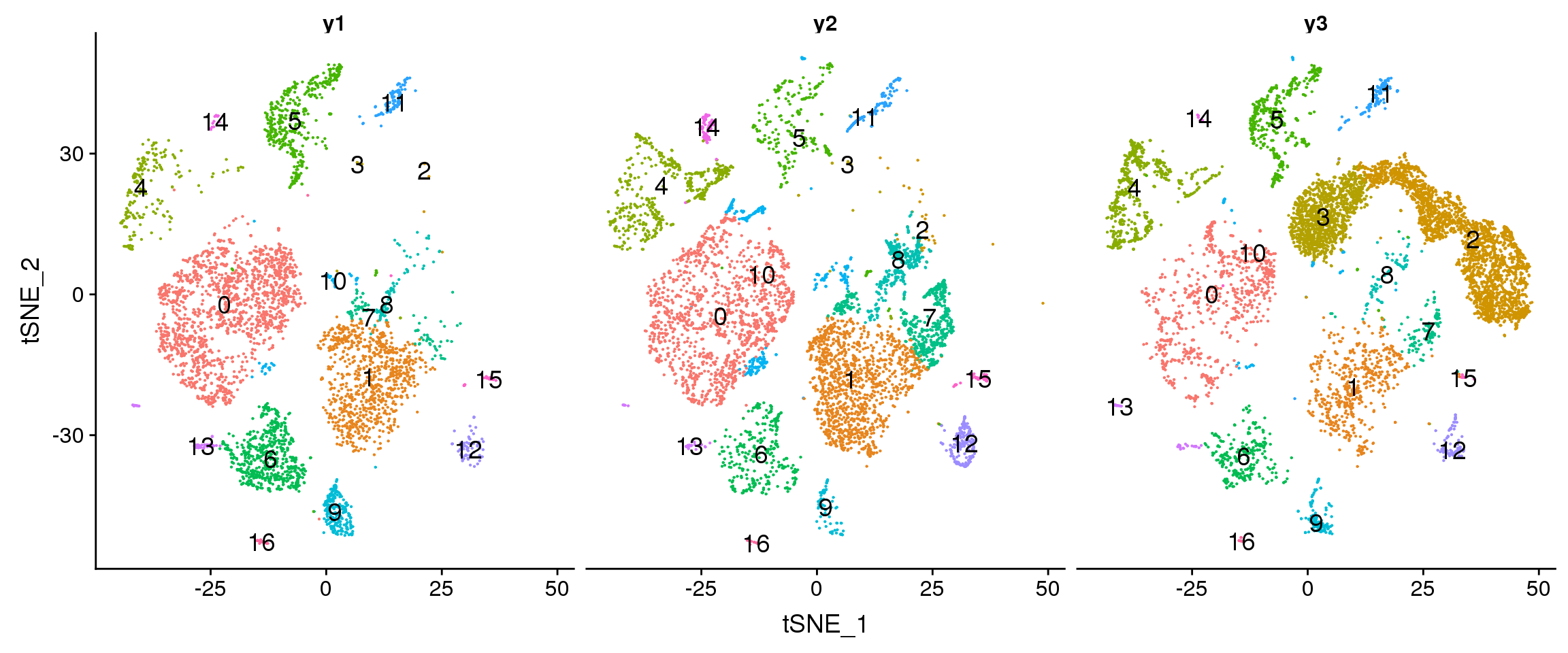
DimPlot(young.integrated, reduction = "tsne", split.by = "sex",label=TRUE,label.size = 5)+NoLegend()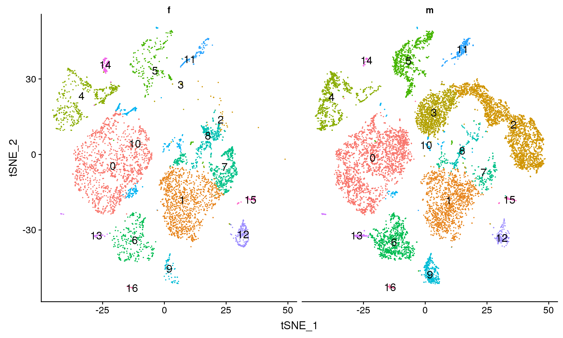
DimPlot(young.integrated, reduction = "tsne", group.by = "biorep")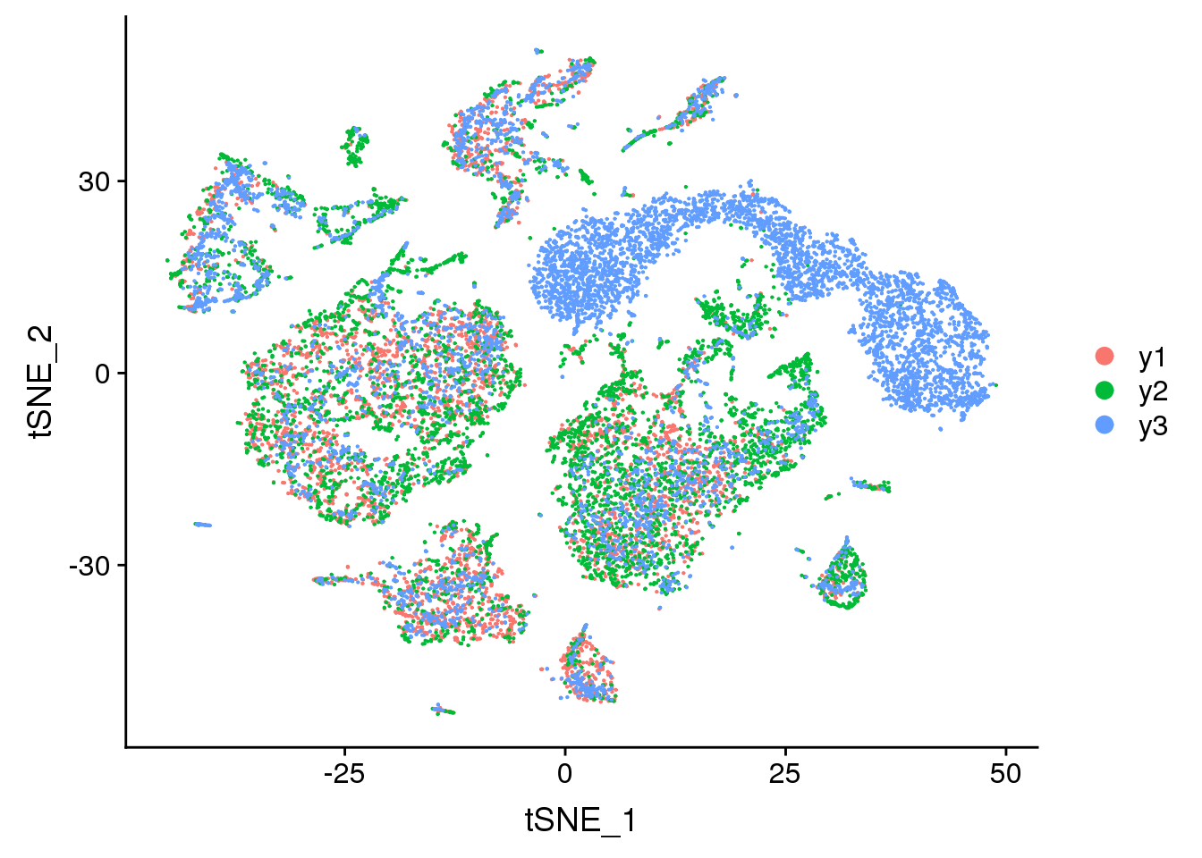
| Version | Author | Date |
|---|---|---|
| b0f9c92 | Belinda Phipson | 2019-07-04 |
DimPlot(young.integrated, reduction = "tsne", group.by = "sex")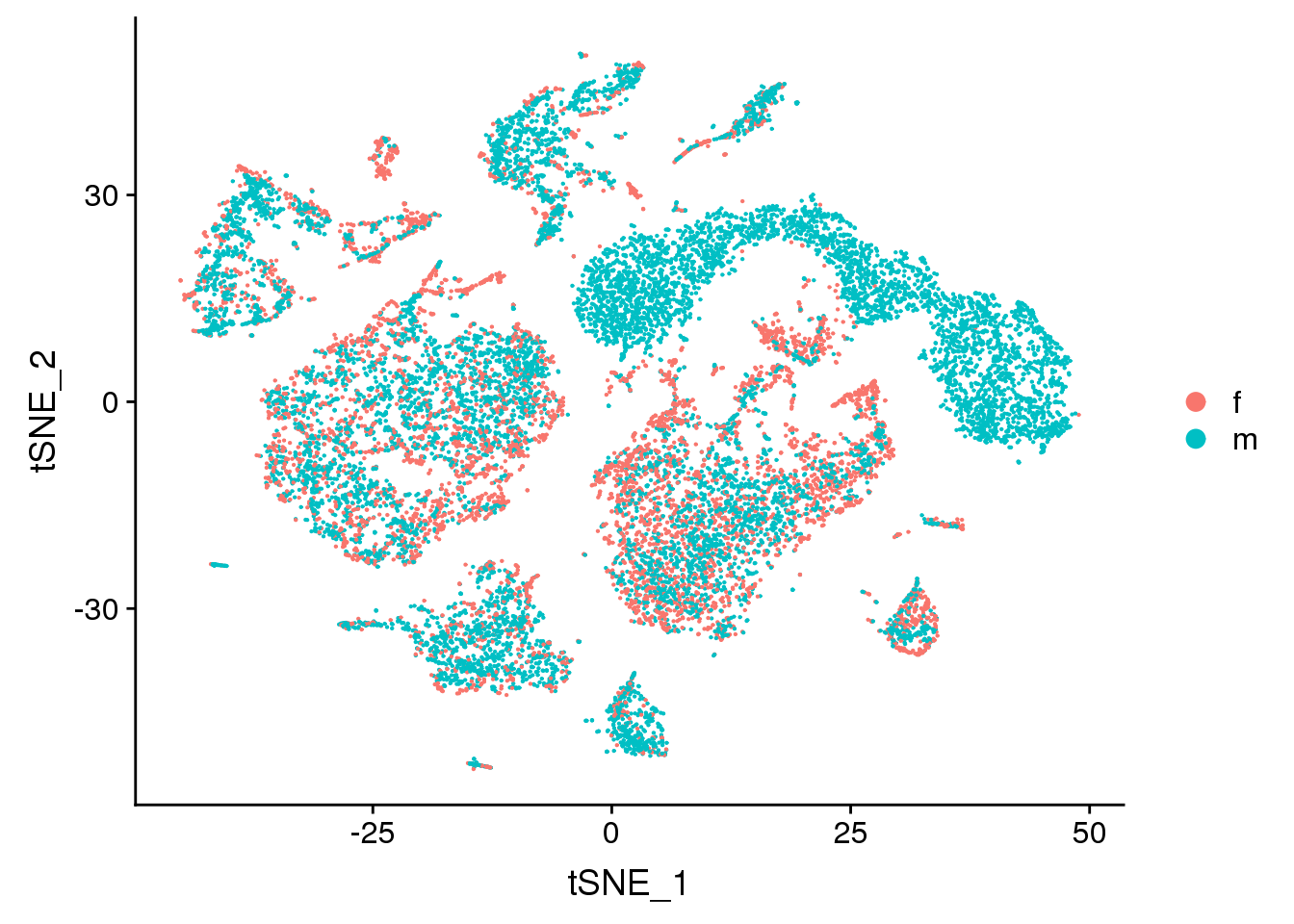
DimPlot(young.integrated, reduction = "tsne", group.by = "batch")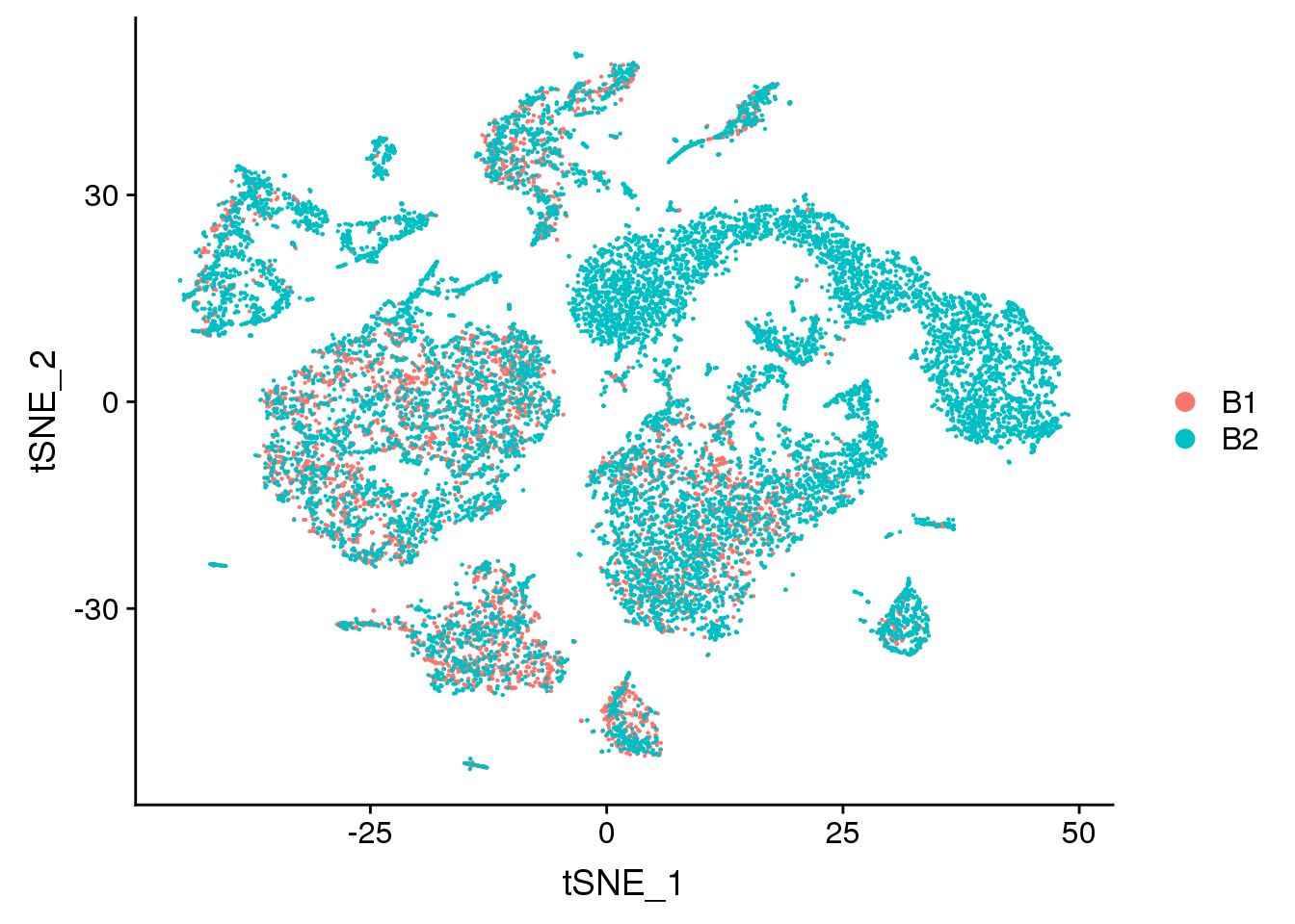
| Version | Author | Date |
|---|---|---|
| b0f9c92 | Belinda Phipson | 2019-07-04 |
DimPlot(young.integrated, reduction = "tsne", group.by = "age")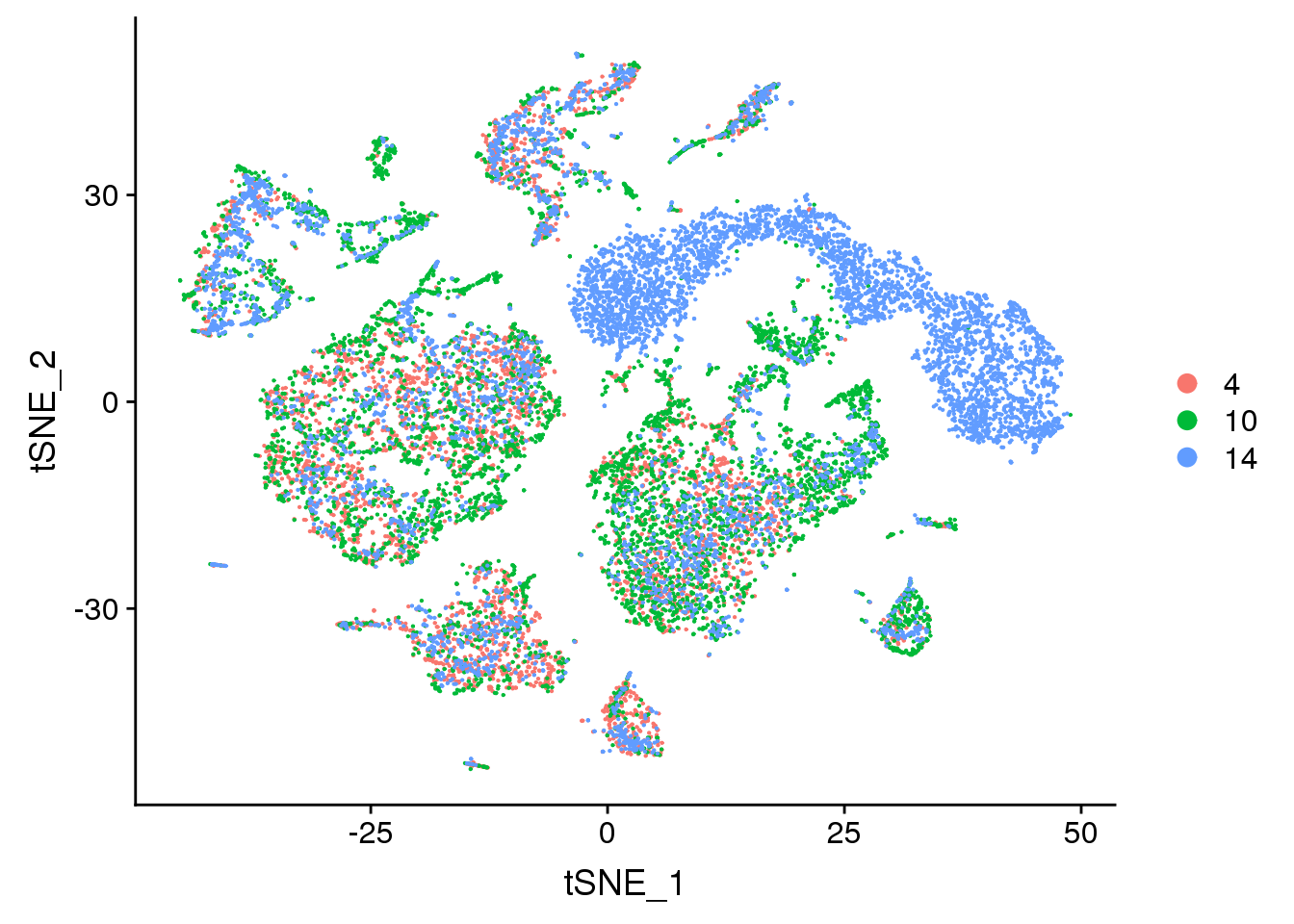
| Version | Author | Date |
|---|---|---|
| b0f9c92 | Belinda Phipson | 2019-07-04 |
FeaturePlot(young.integrated, features = c("TNNT2", "MYH6", "WT1", "PECAM1"), pt.size = 0.2, ncol = 2)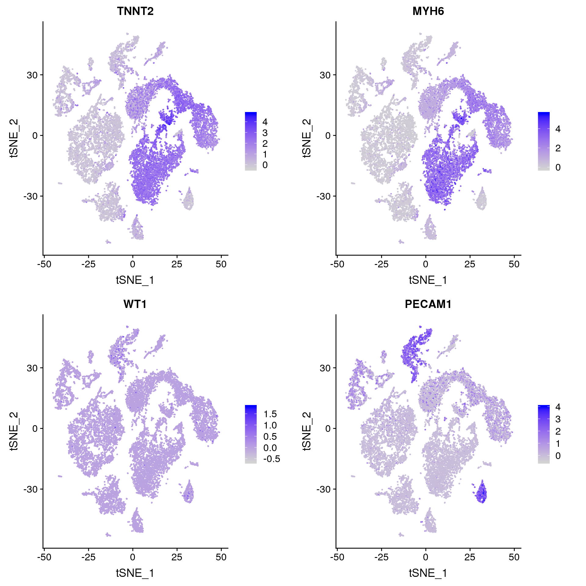
par(mfrow=c(1,1))
par(mar=c(4,4,2,2))
tab <- table(Idents(young.integrated),young@meta.data$biorep)
barplot(t(tab/rowSums(tab)),beside=TRUE,col=ggplotColors(3),legend=TRUE)
| Version | Author | Date |
|---|---|---|
| 45c47f7 | Belinda Phipson | 2019-06-20 |
Visualisation with clustree
clusres <- c(0.1,0.2,0.3,0.4,0.5,0.6,0.7,0.8,0.9,1,1.1,1.2)for(i in 1:length(clusres)){
young.integrated <- FindClusters(young.integrated,
resolution = clusres[i])
}Modularity Optimizer version 1.3.0 by Ludo Waltman and Nees Jan van Eck
Number of nodes: 16964
Number of edges: 692708
Running Louvain algorithm...
Maximum modularity in 10 random starts: 0.9807
Number of communities: 13
Elapsed time: 2 seconds
Modularity Optimizer version 1.3.0 by Ludo Waltman and Nees Jan van Eck
Number of nodes: 16964
Number of edges: 692708
Running Louvain algorithm...
Maximum modularity in 10 random starts: 0.9673
Number of communities: 15
Elapsed time: 2 seconds
Modularity Optimizer version 1.3.0 by Ludo Waltman and Nees Jan van Eck

Number of nodes: 16964
Number of edges: 692708

Running Louvain algorithm...
Maximum modularity in 10 random starts: 0.9543
Number of communities: 17
Elapsed time: 2 seconds
Modularity Optimizer version 1.3.0 by Ludo Waltman and Nees Jan van Eck
Number of nodes: 16964
Number of edges: 692708
Running Louvain algorithm...
Maximum modularity in 10 random starts: 0.9438
Number of communities: 19
Elapsed time: 2 seconds
Modularity Optimizer version 1.3.0 by Ludo Waltman and Nees Jan van Eck
Number of nodes: 16964
Number of edges: 692708
Running Louvain algorithm...
Maximum modularity in 10 random starts: 0.9359
Number of communities: 21
Elapsed time: 2 seconds
Modularity Optimizer version 1.3.0 by Ludo Waltman and Nees Jan van Eck
Number of nodes: 16964
Number of edges: 692708
Running Louvain algorithm...
Maximum modularity in 10 random starts: 0.9283
Number of communities: 23
Elapsed time: 2 seconds
Modularity Optimizer version 1.3.0 by Ludo Waltman and Nees Jan van Eck
Number of nodes: 16964
Number of edges: 692708
Running Louvain algorithm...
Maximum modularity in 10 random starts: 0.9208
Number of communities: 23
Elapsed time: 2 seconds
Modularity Optimizer version 1.3.0 by Ludo Waltman and Nees Jan van Eck
Number of nodes: 16964
Number of edges: 692708
Running Louvain algorithm...
Maximum modularity in 10 random starts: 0.9132
Number of communities: 26
Elapsed time: 2 seconds
Modularity Optimizer version 1.3.0 by Ludo Waltman and Nees Jan van Eck
Number of nodes: 16964
Number of edges: 692708
Running Louvain algorithm...
Maximum modularity in 10 random starts: 0.9075
Number of communities: 27
Elapsed time: 2 seconds
Modularity Optimizer version 1.3.0 by Ludo Waltman and Nees Jan van Eck
Number of nodes: 16964
Number of edges: 692708
Running Louvain algorithm...
Maximum modularity in 10 random starts: 0.9018
Number of communities: 28
Elapsed time: 2 seconds
Modularity Optimizer version 1.3.0 by Ludo Waltman and Nees Jan van Eck
Number of nodes: 16964
Number of edges: 692708
Running Louvain algorithm...
Maximum modularity in 10 random starts: 0.8962
Number of communities: 29
Elapsed time: 2 seconds
Modularity Optimizer version 1.3.0 by Ludo Waltman and Nees Jan van Eck
Number of nodes: 16964
Number of edges: 692708
Running Louvain algorithm...
Maximum modularity in 10 random starts: 0.8912
Number of communities: 30
Elapsed time: 2 secondspct.male <- function(x) {mean(x=="m")}
pct.female <- function(x) {mean(x=="f")}
biorep1 <- function(x) {mean(x=="y1")}
biorep2 <- function(x) {mean(x=="y2")}
biorep3 <- function(x) {mean(x=="y3")}clustree(young.integrated, prefix = "integrated_snn_res.")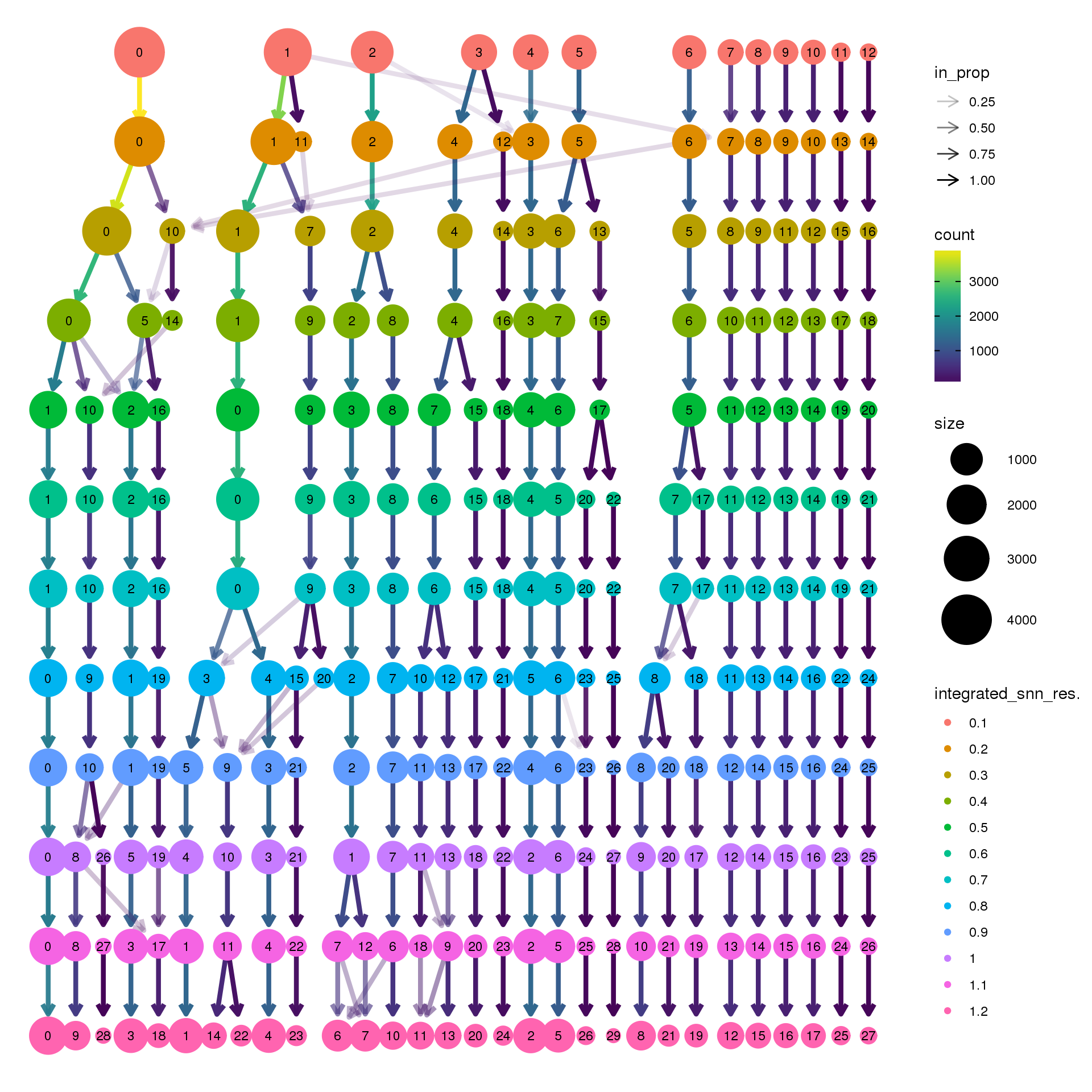
clustree(young.integrated, prefix = "integrated_snn_res.",
node_colour = "biorep", node_colour_aggr = "biorep1",assay="RNA")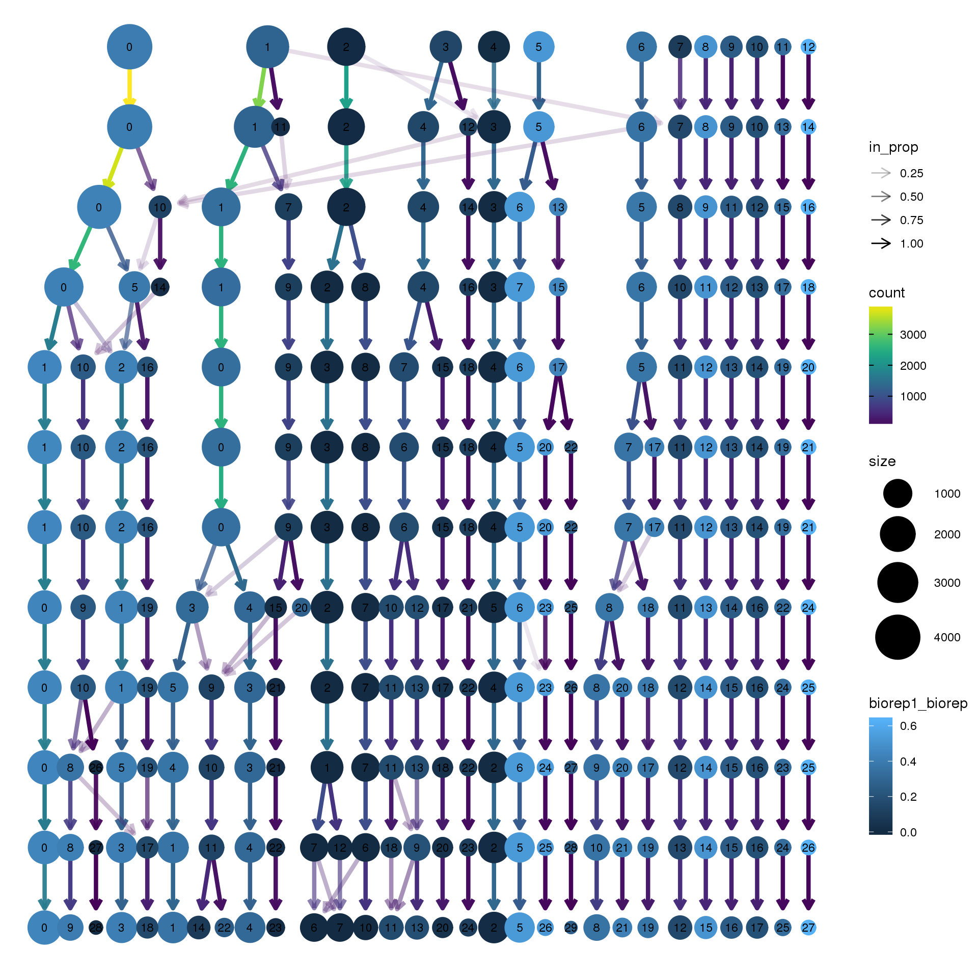
clustree(young.integrated, prefix = "integrated_snn_res.",
node_colour = "biorep", node_colour_aggr = "biorep2",assay="RNA")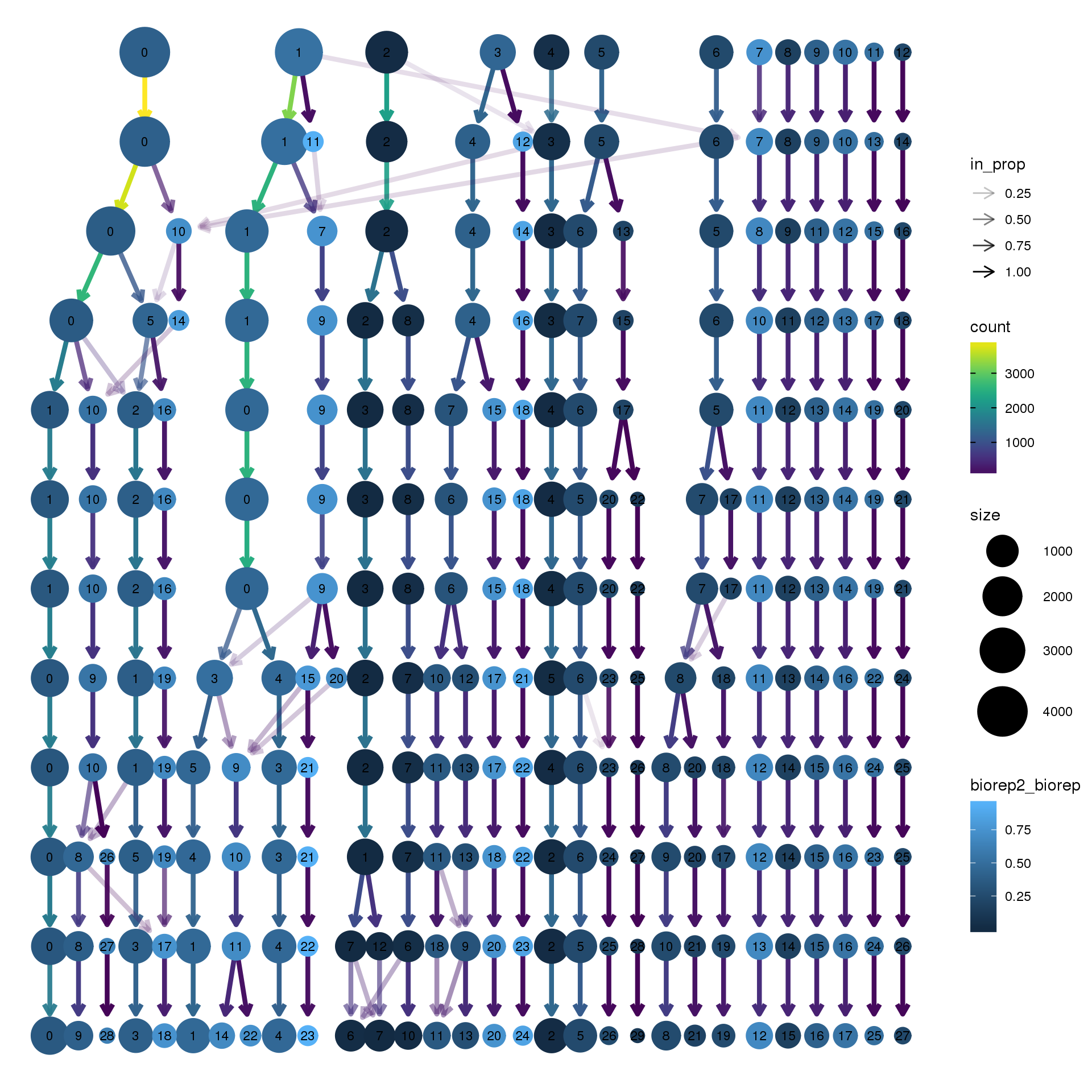
| Version | Author | Date |
|---|---|---|
| b0f9c92 | Belinda Phipson | 2019-07-04 |
clustree(young.integrated, prefix = "integrated_snn_res.",
node_colour = "biorep", node_colour_aggr = "biorep3",assay="RNA")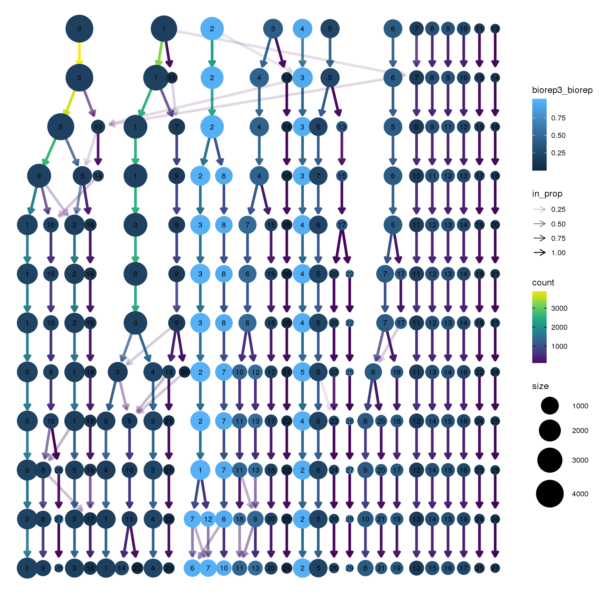
clustree(young.integrated, prefix = "integrated_snn_res.",
node_colour = "sex", node_colour_aggr = "pct.female",assay="RNA")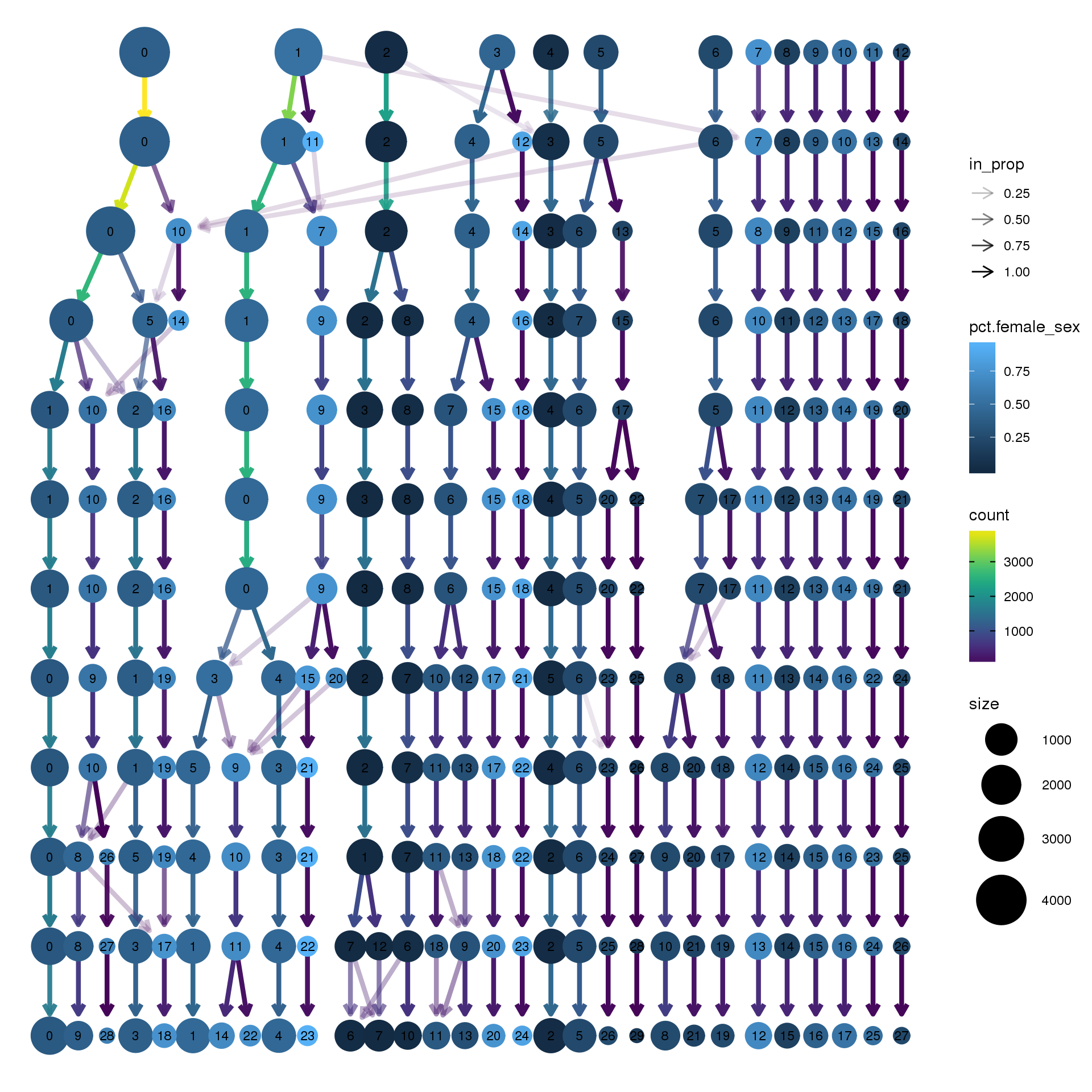
| Version | Author | Date |
|---|---|---|
| b0f9c92 | Belinda Phipson | 2019-07-04 |
clustree(young.integrated, prefix = "integrated_snn_res.",
node_colour = "sex", node_colour_aggr = "pct.male",assay="RNA")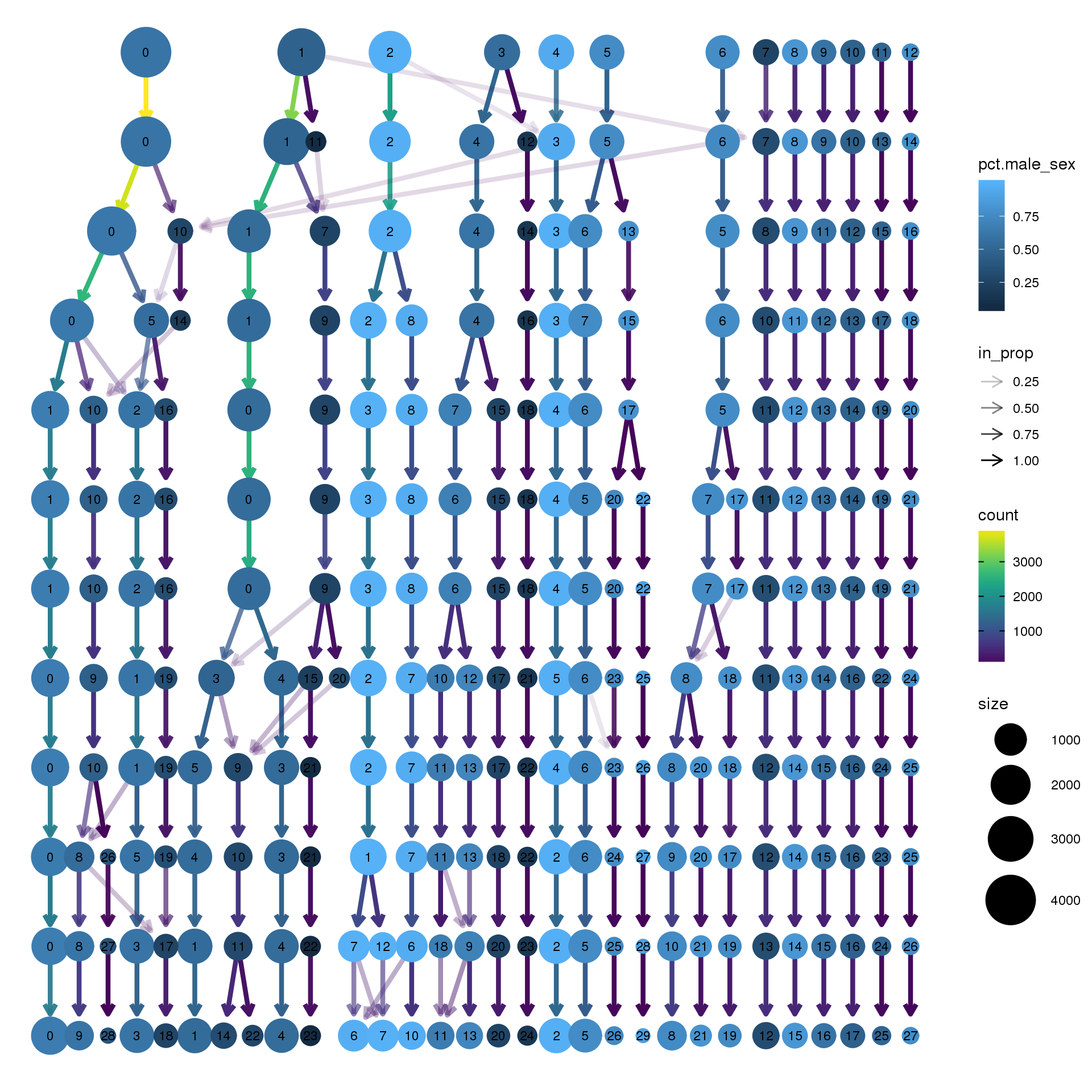
| Version | Author | Date |
|---|---|---|
| 45c47f7 | Belinda Phipson | 2019-06-20 |
#clustree(young.integrated, prefix = "integrated_snn_res.",
# node_colour = "XIST", node_colour_aggr = "median",
# assay="RNA")clustree(young.integrated, prefix = "integrated_snn_res.",
node_colour = "TNNT2", node_colour_aggr = "median",
assay="RNA")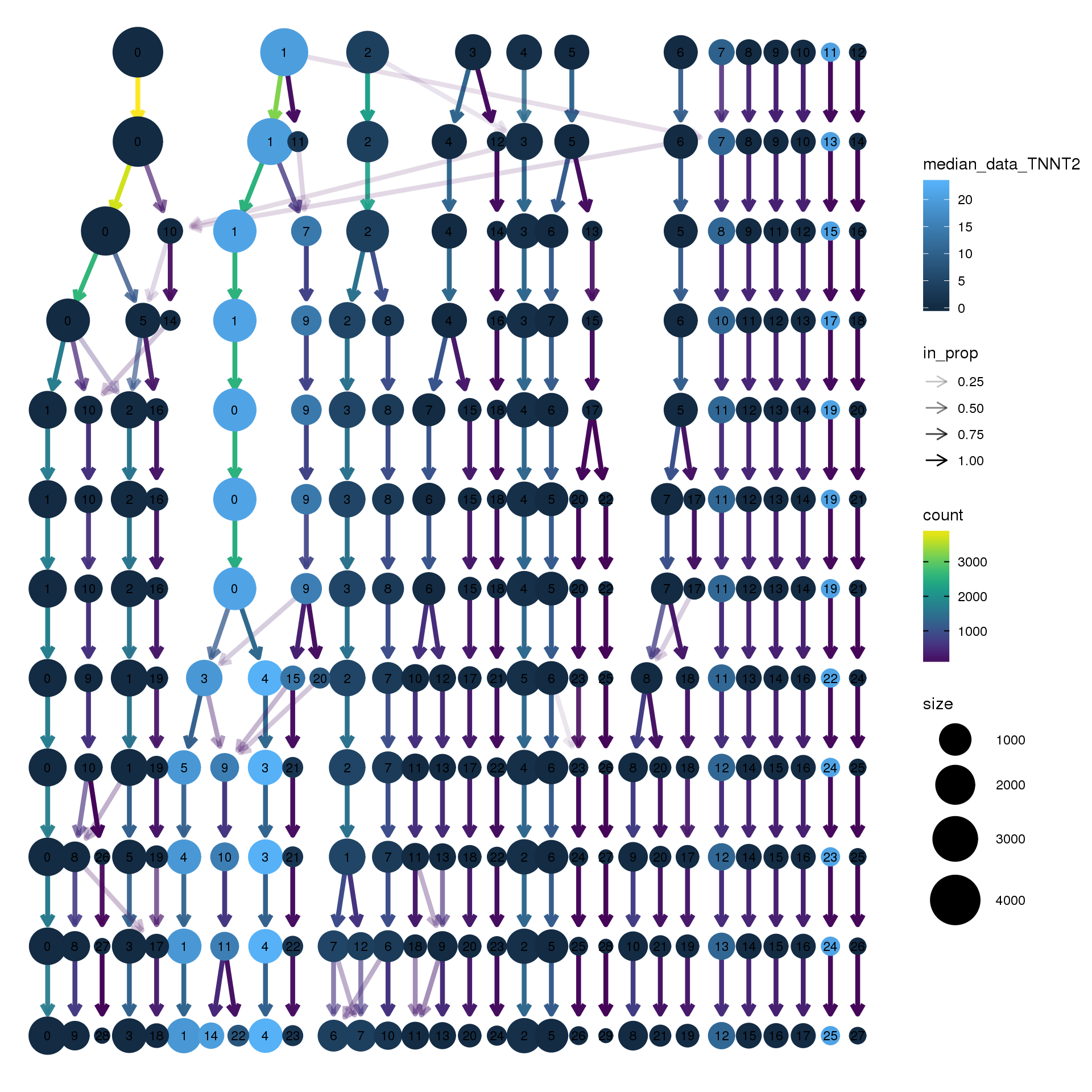
Save Seurat object
DefaultAssay(young.integrated) <- "RNA"
Idents(young.integrated) <- young.integrated$integrated_snn_res.0.3saveRDS(young.integrated,file="./output/RDataObjects/young-int.Rds")
#young.integrated <- readRDS(file="./output/RDataObjects/young-int.Rds")Find Markers
par(mfrow=c(1,1))
par(mar=c(4,4,2,2))
tab <- table(Idents(young.integrated),young@meta.data$biorep)
barplot(t(tab/rowSums(tab)),beside=TRUE,col=ggplotColors(3),legend=TRUE)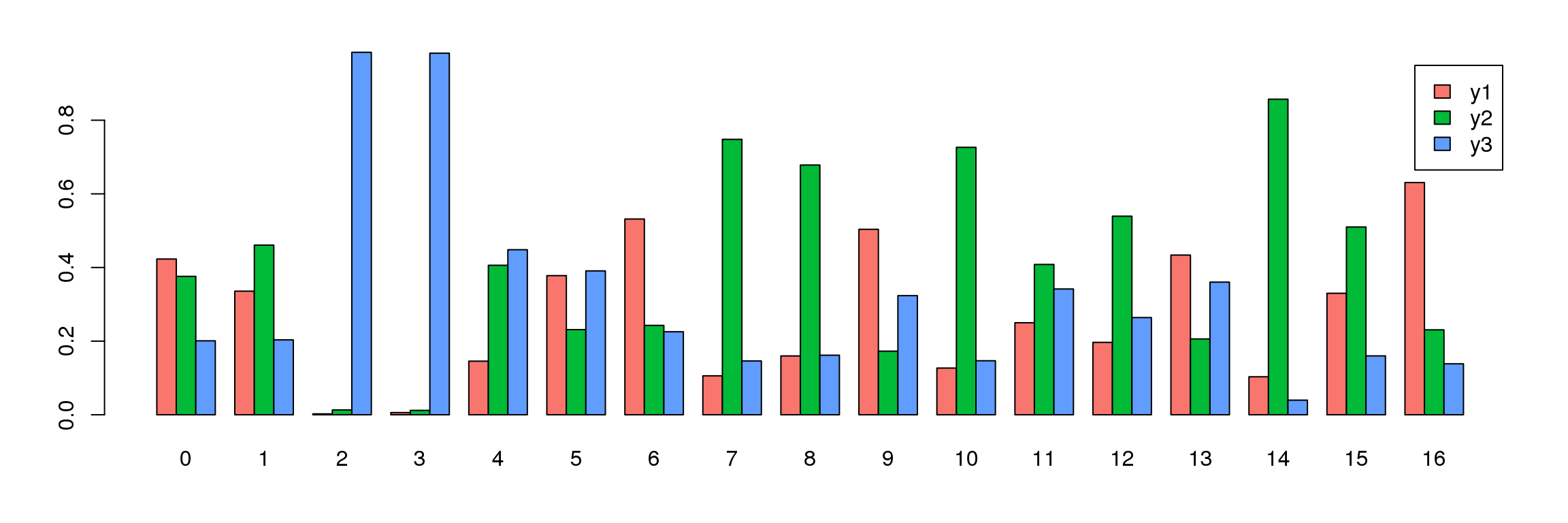
#youngmarkers <- FindAllMarkers(young.integrated, only.pos = TRUE, min.pct = 0.25, logfc.threshold = 0.25)

# Limma-trend for DE

y.young <- DGEList(ally.keep)

logcounts <- normCounts(y.young,log=TRUE,prior.count=0.5)

#logcounts.n <- normalizeBetweenArrays(logcounts, method = "cyclicloess")

maxclust <- length(levels(Idents(young.integrated)))-1

grp <- paste("c",Idents(young.integrated),sep = "")
grp <- factor(grp,levels = paste("c",0:maxclust,sep=""))

design <- model.matrix(~0+grp)
colnames(design) <- levels(grp)

mycont <- matrix(NA,ncol=length(levels(grp)),nrow=length(levels(grp)))
rownames(mycont)<-colnames(mycont)<-levels(grp)
diag(mycont)<-1
mycont[upper.tri(mycont)]<- -1/(length(levels(factor(grp)))-1)
mycont[lower.tri(mycont)]<- -1/(length(levels(factor(grp)))-1)

fit <- lmFit(logcounts,design)
fit.cont <- contrasts.fit(fit,contrasts=mycont)
fit.cont <- eBayes(fit.cont,trend=TRUE,robust=TRUE)

fit.cont$genes <- ann.keep

summary(decideTests(fit.cont))
c0 c1 c2 c3 c4 c5 c6 c7 c8 c9 c10
Down 4891 6788 4196 12699 6430 5061 5085 5098 7642 4783 5751
NotSig 5945 5704 8817 4722 7268 8700 8270 8491 7764 10160 10601
Up 6915 5259 4738 330 4053 3990 4396 4162 2345 2808 1399
c11 c12 c13 c14 c15 c16
Down 5908 2935 1825 2115 610 2635
NotSig 9679 11207 14097 10989 13730 13855
Up 2164 3609 1829 4647 3411 1261treat <- treat(fit.cont,lfc=0.5)
dt <- decideTests(treat)
summary(dt) c0 c1 c2 c3 c4 c5 c6 c7 c8 c9 c10
Down 256 359 3 1201 473 331 310 269 573 329 206
NotSig 16815 16496 17353 16516 16611 16832 16913 16882 16780 16920 17479
Up 680 896 395 34 667 588 528 600 398 502 66
c11 c12 c13 c14 c15 c16
Down 608 231 113 310 18 314
NotSig 16774 16949 17281 16365 17182 17155
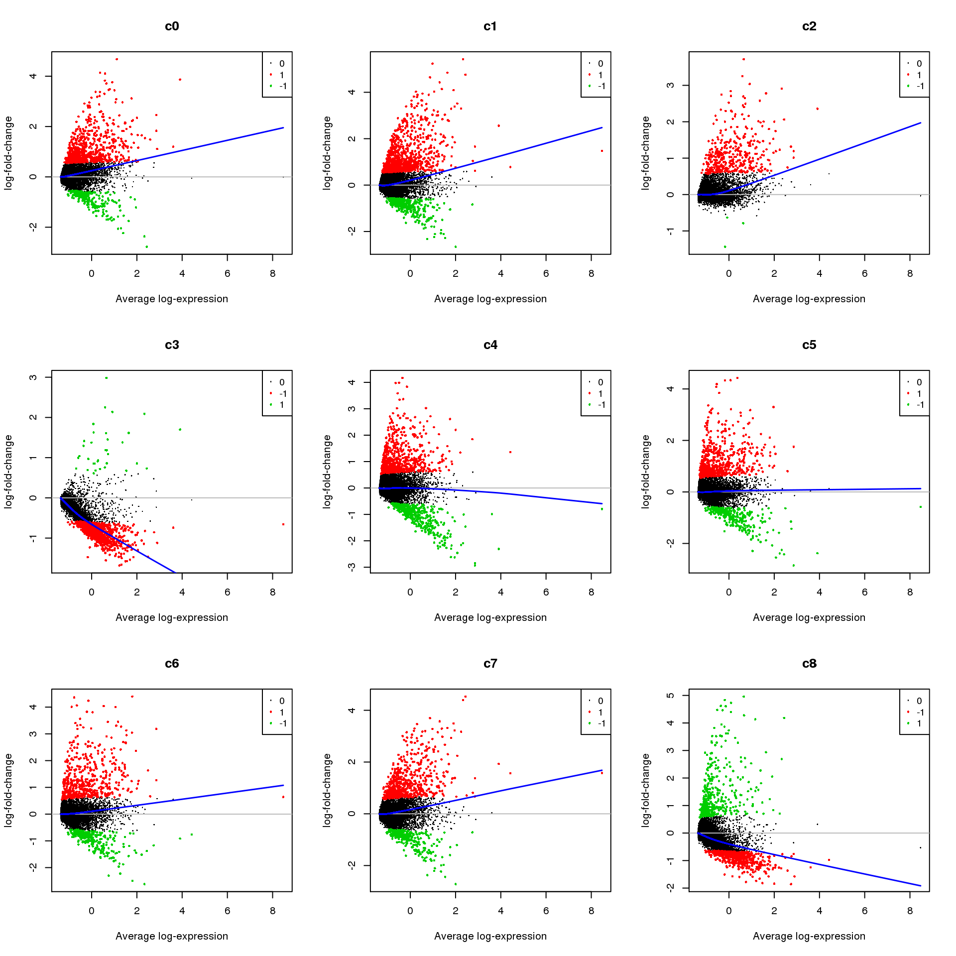
Up 369 571 357 1076 551 282par(mfrow=c(3,3))
for(i in 1:ncol(mycont)){
plotMD(treat,coef=i,status = dt[,i],hl.cex=0.5)
abline(h=0,col=colours()[c(226)])
lines(lowess(treat$Amean,treat$coefficients[,i]),lwd=1.5,col=4)
}
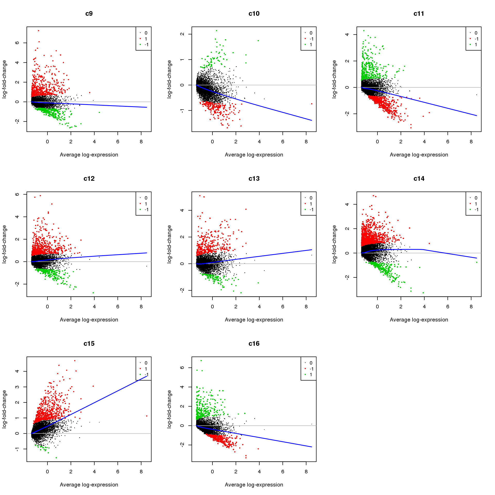
Write out marker genes for each cluster
#write.csv(youngmarkers,file="./output/AllYoung-clustermarkers.csv")contnames <- colnames(mycont)
for(i in 1:length(contnames)){
topsig <- topTreat(treat,coef=i,n=Inf,p.value=0.05)
write.csv(topsig[topsig$logFC>0,],file=paste("./output/MarkerAnalysis/Young/Up-Cluster-",contnames[i],".csv",sep=""))
write.csv(topGO(goana(de=topsig$ENTREZID[topsig$logFC>0],universe=treat$genes$ENTREZID,species="Hs"),number=50),
file=paste("./output/MarkerAnalysis/Young/GO-Cluster-",contnames[i],".csv",sep=""))
}
#write.csv(fetalmarkers,file="./output/AllFetal-clustermarkers.csv")Heatmap of pre-defined heart cell type markers
hm <- read.delim("./data/heart-markers-long.txt",stringsAsFactors = FALSE)
hgene <- toupper(hm$Gene)
hgene <- unique(hgene)

m <- match(hgene,rownames(logcounts))
m <- m[!is.na(m)]

sam <- factor(young.integrated$biorep)
newgrp <- paste(grp,sam,sep=".")
newgrp <- factor(newgrp,levels=paste(rep(levels(grp),each=3),levels(sam),sep="."))
o <-order(newgrp)

annot <- data.frame(CellType=grp,Sample=sam,NewGroup=newgrp)

mycelltypes <- hm$Celltype[match(rownames(logcounts)[m],toupper(hm$Gene))]
mycelltypes <- factor(mycelltypes)


myColors <- list(Clust=NA,Sample=NA,Celltypes=NA)
myColors$Clust<-sample(ggplotColors(length(levels(grp))),length(levels(grp)))
names(myColors$Clust)<-levels(grp)
myColors$Sample <- brewer.pal(3, "Set1")
names(myColors$Sample) <- levels(sam)
myColors$Celltypes <- ggplotColors(length(levels(mycelltypes)))
names(myColors$Celltypes) <- levels(mycelltypes)

mygenes <- rownames(logcounts)[m]
mygenelab <- paste(mygenes,mycelltypes,sep="_")
par(mfrow=c(1,1))
pdf(file="./output/Figures/young-heatmap-hmarkers.pdf",width=20,height=15,onefile = FALSE)
aheatmap(logcounts[m,o],Rowv=NA,Colv=NA,labRow=mygenelab,labCol=NA,
annCol=list(Clust=grp[o],Sample=sam[o]),
# annRow = list(Celltypes=mycelltypes),
annColors = myColors,
fontsize=16,color="-RdYlBu")
dev.off()png
2 Summarise expression across cells
sumexpr <- matrix(NA,nrow=nrow(logcounts),ncol=length(levels(newgrp)))
rownames(sumexpr) <- rownames(logcounts)
colnames(sumexpr) <- levels(newgrp)

for(i in 1:nrow(sumexpr)){
  sumexpr[i,] <- tapply(logcounts[i,],newgrp,median)
}
par(mfrow=c(1,1))
clust <- rep(levels(grp),each=3)
samps <- rep(levels(sam),length(levels(grp)))
pdf(file="./output/Figures/young-heatmap-hmarkers-summarised.pdf",width=20,height=15,onefile = FALSE)
aheatmap(sumexpr[m,],Rowv = NA,Colv = NA, labRow = mygenelab,
annCol=list(Clust=clust,Sample=samps),
# annRow=list(Celltypes=mycelltypes),
annColors=myColors,
fontsize=14,color="-RdYlBu")
dev.off()png
2 aheatmap(sumexpr[m,],Rowv = NA,Colv = NA, labRow = mygenelab,
annCol=list(Clust=clust,Sample=samps),
# annRow=list(Celltypes=mycelltypes),
annColors=myColors,
fontsize=12,color="-RdYlBu")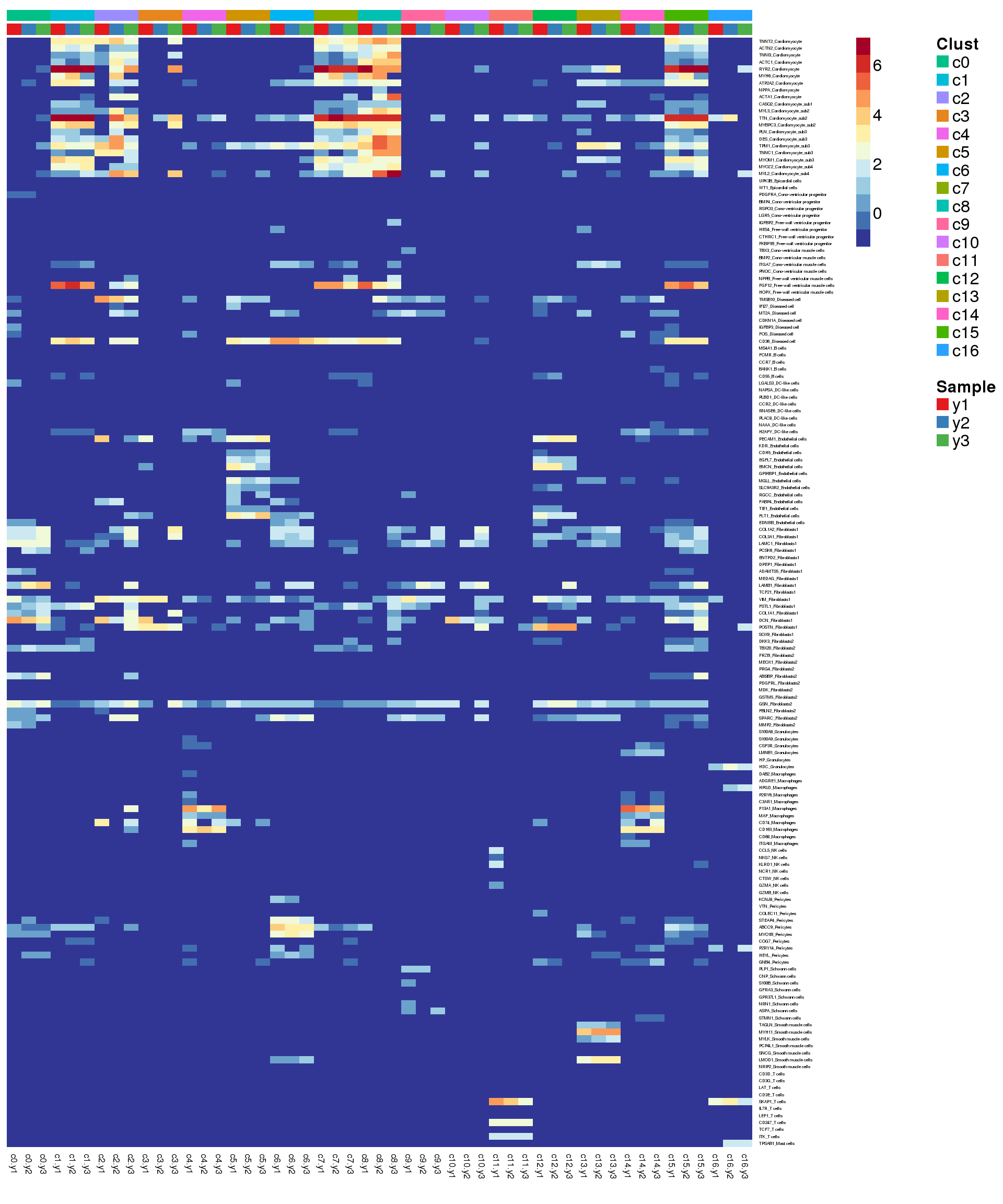
sig.genes <- gene.label <- vector("list", length(levels(grp)))
for(i in 1:length(sig.genes)){
  top <- topTreat(treat,coef=i,n=200)
  sig.genes[[i]] <- rownames(top)[top$logFC>0][1:5]
  gene.label[[i]] <- paste(rownames(top)[top$logFC>0][1:5],levels(grp)[i],sep="-")
}

csig <- unlist(sig.genes)
genes <- unlist(gene.label)

pdf(file="./output/Figures/young-heatmap-siggenes-summarised.pdf",width=20,height=15,onefile = FALSE)
aheatmap(sumexpr[csig,],Rowv = NA,Colv = NA, labRow = genes,
         annCol=list(Clust=clust,Sample=samps),
         annColors=myColors,
         fontsize=16,color="-RdYlBu",
         scale="none")
dev.off()
png
2 aheatmap(sumexpr[csig,],Rowv = NA,Colv = NA, labRow = genes,
annCol=list(Clust=clust,Sample=samps),
annColors=myColors,
fontsize=16,color="-RdYlBu",
scale="none")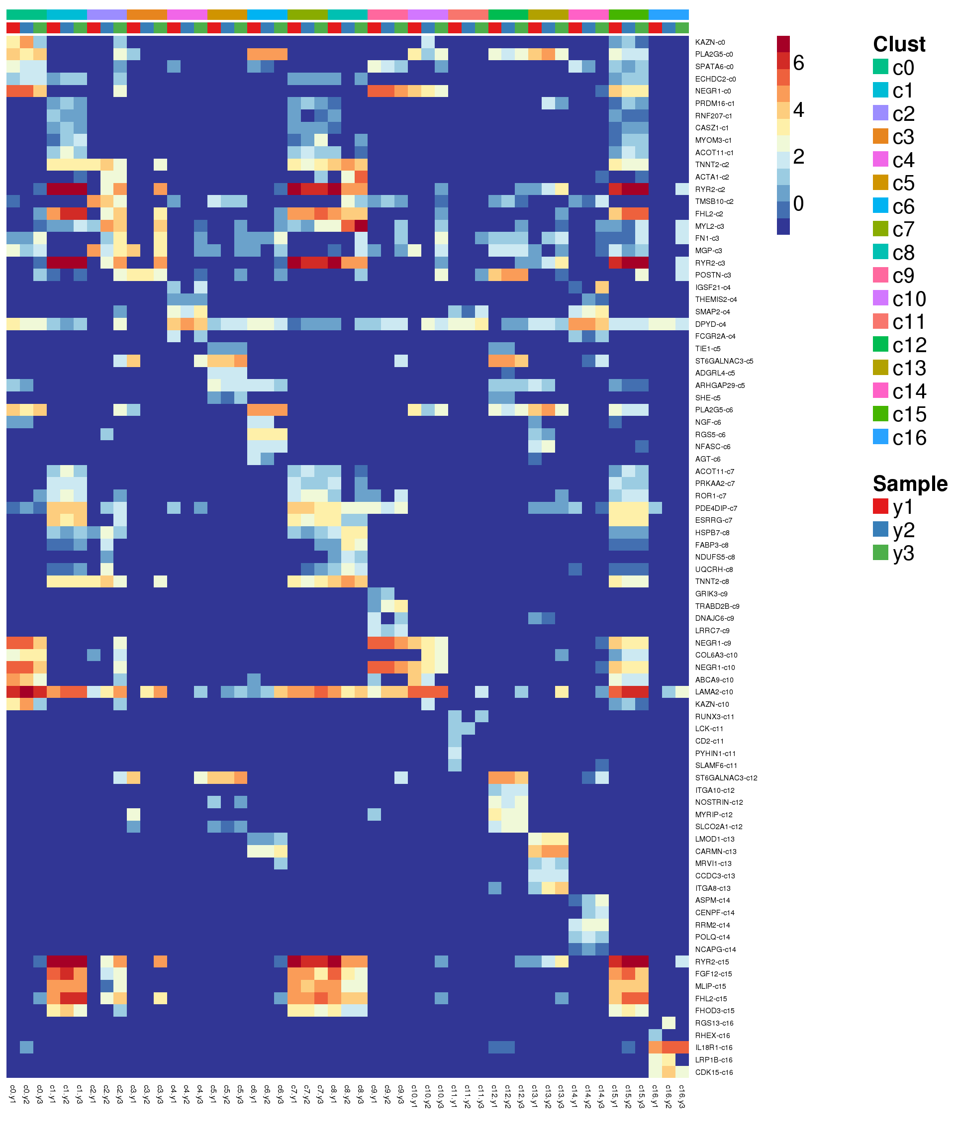
Try annotate clusters based on fetal cell types
# This loads a list object called sig.genes.gst
load(file="./data/gstlist-fetal.Rdata")

expr.score <- matrix(NA,nrow=length(sig.genes.gst),ncol=length(levels(newgrp)))
colnames(expr.score) <- levels(newgrp)
rownames(expr.score) <- names(sig.genes.gst)

specialm <- lapply(sig.genes.gst,function(x) match(x,rownames(sumexpr))[!is.na(match(x,rownames(sumexpr)))])

for(i in 1:nrow(expr.score)){
  expr.score[i,] <- colMeans(sumexpr[specialm[[i]],])
}

pdf(file="./output/Figures/heatmap-match-fetal-young.pdf",width=20,height=15,onefile = FALSE)
aheatmap(expr.score,
         Rowv = NA,Colv = NA,
         labRow = rownames(expr.score),
         annCol=list(Clust=clust,Sample=samps),
         annColors=myColors,
         fontsize=16,color="-RdYlBu",
         scale="none")
dev.off()
png
2 aheatmap(expr.score,
# Rowv = NA,Colv = NA,
labRow = rownames(expr.score),
annCol=list(Clust=clust,Sample=samps),
annColors=myColors,
fontsize=16,color="-RdYlBu",
scale="none")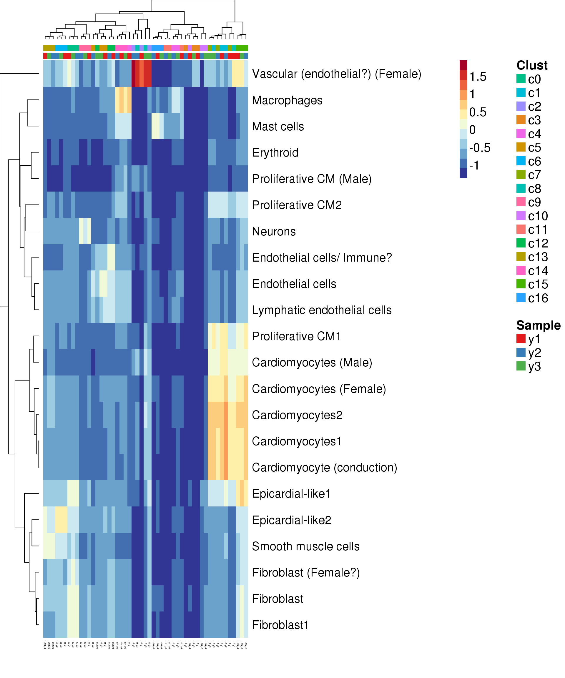
avgexp <- matrix(NA,nrow=nrow(logcounts),ncol=length(levels(grp)))
rownames(avgexp) <- rownames(logcounts)
colnames(avgexp) <- levels(grp)
for(i in 1:nrow(avgexp)) avgexp[i,] <- tapply(logcounts[i,],grp,mean)

pdf(file="./output/Figures/avgcl-exp-young.pdf",width=10,height=10)
par(mfrow=c(3,3))
for(i in 1:9){
  plot(treat$Amean,avgexp[,i],pch=16,cex=0.5,col=rgb(0,0,1,alpha=0.4),main=colnames(avgexp)[i])
  abline(a=0,b=1,col=1)
}
dev.off()
png
2 pdf(file="./output/Figures/avgcl-exp2-young.pdf",width=10,height=10)
par(mfrow=c(3,3))
for(i in 10:length(levels(grp))){
plot(treat$Amean,avgexp[,i],pch=16,cex=0.5,col=rgb(0,0,1,alpha=0.4),main=colnames(avgexp)[i])
abline(a=0,b=1,col=1)
}
dev.off()png
2 min(avgexp)[1] -1.372213pdf(file="./output/Figures/avgcl-exp-boxplot-young.pdf",width=10,height=10)
par(mfrow=c(1,1))
boxplot(avgexp,ylim=c(min(avgexp),2))
dev.off()png
2 Create list of marker genes for GST purposes
young.sig.genes.gst <- vector("list", length(levels(grp)))
names(young.sig.genes.gst) <- levels(grp)
for(i in 1:length(young.sig.genes.gst)){
  top <- topTreat(treat,coef=i,n=Inf,p.value=0.05)
  young.sig.genes.gst[[i]] <- rownames(top)[top$logFC>0]
}
save(young.sig.genes.gst,file="./data/gstlist-young.Rdata")
sessionInfo()R version 3.6.0 (2019-04-26)
Platform: x86_64-pc-linux-gnu (64-bit)
Running under: CentOS release 6.7 (Final)
Matrix products: default
BLAS: /usr/local/installed/R/3.6.0/lib64/R/lib/libRblas.so
LAPACK: /usr/local/installed/R/3.6.0/lib64/R/lib/libRlapack.so
locale:
[1] LC_CTYPE=en_US.UTF-8 LC_NUMERIC=C
[3] LC_TIME=en_US.UTF-8 LC_COLLATE=en_US.UTF-8
[5] LC_MONETARY=en_US.UTF-8 LC_MESSAGES=en_US.UTF-8
[7] LC_PAPER=en_US.UTF-8 LC_NAME=C
[9] LC_ADDRESS=C LC_TELEPHONE=C
[11] LC_MEASUREMENT=en_US.UTF-8 LC_IDENTIFICATION=C
attached base packages:
[1] splines parallel stats4 stats graphics grDevices utils
[8] datasets methods base
other attached packages:
[1] dplyr_0.8.1 clustree_0.4.0
[3] ggraph_1.0.2 workflowr_1.3.0
[5] NMF_0.21.0 bigmemory_4.5.33
[7] cluster_2.0.9 rngtools_1.3.1.1
[9] pkgmaker_0.27 registry_0.5-1
[11] scran_1.12.0 SingleCellExperiment_1.6.0
[13] SummarizedExperiment_1.14.0 GenomicRanges_1.36.0
[15] GenomeInfoDb_1.20.0 DelayedArray_0.10.0
[17] BiocParallel_1.18.0 matrixStats_0.54.0
[19] cowplot_0.9.4 monocle_2.12.0
[21] DDRTree_0.1.5 irlba_2.3.3
[23] VGAM_1.1-1 ggplot2_3.1.1
[25] Matrix_1.2-17 Seurat_3.0.2
[27] org.Hs.eg.db_3.8.2 AnnotationDbi_1.46.0
[29] IRanges_2.18.0 S4Vectors_0.22.0
[31] Biobase_2.44.0 BiocGenerics_0.30.0
[33] RColorBrewer_1.1-2 edgeR_3.26.3
[35] limma_3.40.2
loaded via a namespace (and not attached):
[1] reticulate_1.12 R.utils_2.8.0
[3] tidyselect_0.2.5 RSQLite_2.1.1
[5] htmlwidgets_1.3 grid_3.6.0
[7] combinat_0.0-8 docopt_0.6.1
[9] Rtsne_0.15 munsell_0.5.0
[11] codetools_0.2-16 ica_1.0-2
[13] statmod_1.4.30 future_1.12.0
[15] withr_2.1.2 colorspace_1.4-1
[17] fastICA_1.2-1 knitr_1.22
[19] ROCR_1.0-7 gbRd_0.4-11
[21] listenv_0.7.0 Rdpack_0.11-0
[23] labeling_0.3 git2r_0.25.2
[25] slam_0.1-45 GenomeInfoDbData_1.2.1
[27] polyclip_1.10-0 bit64_0.9-7
[29] farver_1.1.0 pheatmap_1.0.12
[31] rprojroot_1.3-2 xfun_0.6
[33] R6_2.4.0 doParallel_1.0.14
[35] ggbeeswarm_0.6.0 rsvd_1.0.0
[37] locfit_1.5-9.1 bitops_1.0-6
[39] assertthat_0.2.1 SDMTools_1.1-221.1
[41] scales_1.0.0 beeswarm_0.2.3
[43] gtable_0.3.0 npsurv_0.4-0
[45] globals_0.12.4 tidygraph_1.1.2
[47] rlang_0.3.4 lazyeval_0.2.2
[49] checkmate_1.9.3 yaml_2.2.0
[51] reshape2_1.4.3 backports_1.1.4
[53] tools_3.6.0 gridBase_0.4-7
[55] gplots_3.0.1.1 dynamicTreeCut_1.63-1
[57] ggridges_0.5.1 Rcpp_1.0.1
[59] plyr_1.8.4 zlibbioc_1.30.0
[61] purrr_0.3.2 RCurl_1.95-4.12
[63] densityClust_0.3 pbapply_1.4-0
[65] viridis_0.5.1 zoo_1.8-5
[67] ggrepel_0.8.1 fs_1.3.1
[69] magrittr_1.5 data.table_1.11.6
[71] lmtest_0.9-37 RANN_2.6.1
[73] whisker_0.3-2 fitdistrplus_1.0-14
[75] lsei_1.2-0 evaluate_0.13
[77] xtable_1.8-4 sparsesvd_0.1-4
[79] gridExtra_2.3 HSMMSingleCell_1.4.0
[81] compiler_3.6.0 scater_1.12.2
[83] tibble_2.1.1 KernSmooth_2.23-15
[85] crayon_1.3.4 R.oo_1.22.0
[87] htmltools_0.3.6 tidyr_0.8.3
[89] DBI_1.0.0 tweenr_1.0.1
[91] MASS_7.3-51.4 R.methodsS3_1.7.1
[93] gdata_2.18.0 metap_1.1
[95] igraph_1.2.4.1 pkgconfig_2.0.2
[97] bigmemory.sri_0.1.3 plotly_4.9.0
[99] foreach_1.4.4 vipor_0.4.5
[101] dqrng_0.2.1 XVector_0.24.0
[103] bibtex_0.4.2 stringr_1.4.0
[105] digest_0.6.18 sctransform_0.2.0
[107] tsne_0.1-3 rmarkdown_1.12.6
[109] DelayedMatrixStats_1.6.0 gtools_3.8.1
[111] nlme_3.1-139 jsonlite_1.6
[113] BiocNeighbors_1.2.0 viridisLite_0.3.0
[115] pillar_1.3.1 lattice_0.20-38
[117] GO.db_3.8.2 httr_1.4.0
[119] survival_2.44-1.1 glue_1.3.1
[121] qlcMatrix_0.9.7 FNN_1.1.3
[123] png_0.1-7 iterators_1.0.10
[125] bit_1.1-14 ggforce_0.2.2
[127] stringi_1.4.3 blob_1.1.1
[129] BiocSingular_1.0.0 caTools_1.17.1.2
[131] memoise_1.1.0 future.apply_1.2.0
[133] ape_5.3